3.7: A Heuristic View of the Probability Density Function

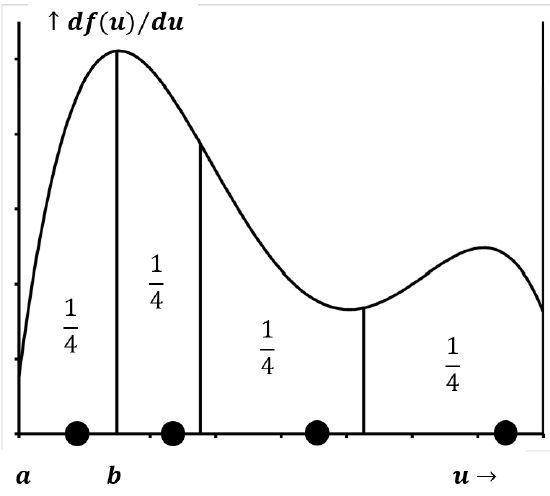
Suppose that we have a probability density function like that sketched in Figure 8 and that the area under the curve in the interval \(a<u<b\) is 0.25. If we draw a large number of samples from the distribution, our definitions of probability and the probability density function mean that about 25% of the values we draw will lie in the interval \(a<u<b\). We expect the percentage to become closer and closer to 25% as the total number of samples drawn becomes very large. The same would be true of any other interval, \(c<u<d\), where the area under the curve in the interval \(c<u<d\) is 0.25.

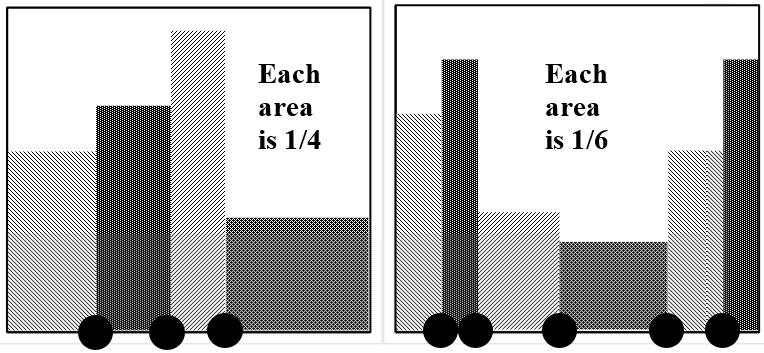
If we draw exactly four samples from this distribution, the values can be anywhere in the domain of \(u\). However, if we ask what arrangement of four values best approximates the result of drawing a large number of samples, it is clear that this arrangement must have a value in each of the four, mutually-exclusive, 25% probability zones. We can extend this conclusion to any number of representative points. If we ask what arrangement of N points would best represent the arrangement of a large number of points drawn from the distribution, the answer is clearly that one of the \(N\) representative points should lie within each of \(N\), mutually-exclusive, equal-area segments that span the domain of \(u\).)

Figure 8. A sample of four that approximates its distribution.

We can turn this idea around. In the absence of information to the contrary, the best assumption we can make about a set of \(N\) values of a random variable is that each represents an equally probable outcome. If our entire store of information about a distribution consists of four data points drawn from the distribution, the best description that we can give of the probability density function is that one-fourth of the area under the curve lies above a segment of the domain that is associated with each point. If we have \(N\) points, the best estimate we can make of the distribution from which the \(N\) points are drawn is that \({\left({1}/{N}\right)}^{th}\) of the area lies above each of them.

This view tells us to associate a probability of \({1}/{N}\) with an interval around each data point, but it does not tell us where to begin or end the interval. If we could decide where the interval about each data point began and ended, we could estimate the shape of the probability density function. For a small number of points, we could not expect this estimate to be very accurate, but it would be the best possible estimate based on the given data.

Figure 9. The sample of four that best approximates its distribution.

Now, instead of trying to find the best interval to associate with each data point, let us think about the intervals into which the data points divide the domain. This small change of perspective leads us to a logical way to divide the domain of \(u\) into specific intervals of equal probability. If we put \(N\) points on any line, these points divide the line into \(N+1\) segments. There is a segment to the left of every point; there are \(N\) such segments. There is one final segment to the right of the right-most point, and so there are \(N+1\) segments in all.

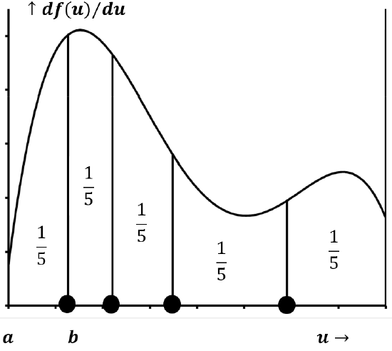
In the absence of information to the contrary, the best assumption we can make is that \(N\) data points divide their domain into \(N+1\) segments, each of which is associated with equal probability. The fraction of the area above each of these segments is \({1}/{\left(N+1\right)}\); also, the probability associated with each segment is \({1}/{\left(N+1\right)}\). If, as in the example above, there are four data points, the best assumption we can make about the probability density function is that 20% of its area lies between the left boundary and the left-most data point, and 20% lies between the right-most data point and the right boundary. The three intervals between the four data points each represent an additional 20% of the area. Figure 9 indicates the \(N\) data points that best approximate the distribution sketched in Figure 8.

The sketches in Figure 10 describe the probability density functions implied by the indicated sets of data points.

Figure 10. Approximate probability density functions.