7.2: Entropic Elasticity

Ideal Chain Model

Most polymer chains have rotatable bonds as well as bond angles along the polymer backbone that differ from 180\(^\circ\). This leads to flexibility of the chain. Even if the rotations are not free, but give rise to only \(n_\mathrm{rot}\) rotameric states per rotatable bond, the number of possible chain conformations becomes vast. For \(N_{rot}\) rotatable bonds, the number of distinct conformations is \(n_\mathrm{rot}^{N_\mathrm{rot}}\). The simplest useful model for such a flexible chain is the freely jointed chain model. Here we assume bond vectors that all have the same length \(l = |\vec{r}_i|\), where \(\vec{r}_i\) is the bond vector of the \(i^\mathrm{th}\) bond. If we further assume an angle \(\theta_{ij}\) between consecutive bond vectors, we can write the scalar product of consecutive bond vectors as

\[\vec{r}_i \cdot \vec{r}_j = l^2 \cos \theta_{ij} \ . \label{eq:fjc_cons}\]

This scalar product is of interest, as we can use it to compute the mean-square end-to-end distance \(\langle R^2 \rangle\) of an ensemble of chains, which is the simplest parameter that characterizes the spatial dimension of the chain. With the end-to-end distance vector of a chain with \(n\) bonds,

\[\vec{R}_n = \sum_{i=1}^n \vec{r}_i \ ,\]

we have

\[\begin{align} \langle R^2 \rangle & = \langle \vec{R}_n^2 \rangle \\ & = \langle \vec{R}_n \cdot \vec{R}_n \rangle \\ & = \left\langle \left( \sum_{i=1}^n \vec{r}_i \right) \cdot \left( \sum_{j=1}^n \vec{r}_j \right) \right\rangle \\ & = \sum_{i=1}^n \sum_{j=1}^n \langle \vec{r}_i \cdot \vec{r}_j \rangle \ .\end{align}\]

By using Equation \ref{eq:fjc_cons}) we find

\[\langle R^2 \rangle = l^2 \sum_{i=1}^n \sum_{j=1}^n \langle \cos \theta_{ij} \rangle \ . \label{eq:fjc_double_sum}\]

In the freely jointed chain model we further assume that there are no correlations between the directions of different bond vectors, \(\langle \cos \theta_{ij} \rangle = 0\) for \(i \neq j\). Then, the double sum in Equation \ref{eq:fjc_double_sum}) has only \(n\) non-zero terms for \(i=j\) with \(\cos \theta_{ij} = 1\). Hence,

\[\langle R^2 \rangle = n l^2 \ . \label{eq:eer_fjc}\]

This again appears to be a crude model, but we shall now rescue it by redefining \(l\). In an ideal polymer chain we can at least assume that there is no interaction between monomers that are separated by many other monomers,

\[\lim\limits_{|i-j| \rightarrow \infty} \langle \cos \theta_{ij} \rangle = 0 \ .\]

Furthermore, for a given bond vector \(\vec{r}_i\) the sum over all correlations with other bond vectors converges to some finite number that depends on \(i\),

\[\sum_{j=1}^n \langle \cos \theta_{ij} \rangle = C'(i) \ .\]

Therefore, when including the correlations, Equation \ref{eq:fjc_double_sum}) can still be simplified to

\[\langle R^2 \rangle = l^2 \sum_{i=1}^n C'(i) = C_n n l^2 \ ,\]

where Flory’s characteristic ratio \(C_n\) is the average value of \(C'(i)\) over all backbone bonds of the chain.

In general, \(C_n\) depends on \(n\), but for very long chains it converges to a value \(C_\infty\). For sufficiently long chains, we can thus approximate

\[\langle R^2 \rangle \approx n C_\infty l^2 \ ,\]

which has the same dependence on \(n\) and \(l\) as the crude model of the freely jointed chain, Equation \ref{eq:eer_fjc}). Hence, we can define an equivalent freely jointed chain with \(N\) Kuhn segments of length \(b\). From

\[\langle R^2 \rangle = N b^2 \approx n C_\infty l^2 \label{eq:Kuhn_R2}\]

and the length of the maximally stretched equivalent chain, the contour length \(R_\mathrm{max}\),

\[R_\mathrm{max} = N b \ ,\]

we obtain

\[N = \frac{R_\mathrm{max}^2}{C_\infty n l^2}\]

and the Kuhn length

\[b = \frac{\langle R^2 \rangle}{R_\mathrm{max}} = \frac{C_\infty n l^2}{R_\mathrm{max}} \ .\]

Typical values of \(C_\infty\) for synthetic polymers range from 4.6 for 1,4-poly(isoprene) to 9.5 for atactic poly(styrene) with corresponding Kuhn lengths of 8.2 Å to 18 Å, respectively.

At this point we have found the mean-square end-to-end distance as a parameter of an equilibrium macrostate. If we stretch the chain to a longer end-to-end distance, it is no longer at equilibrium and must have larger free energy. Part of this increase in free energy must come from a decrease in entropy that stretching induces by reducing the number of accessible chain conformations. It turns out that this entropic contribution is the major part of the increase in free energy, typically 90%. The tendency of polymer chains to contract after they have been stretched is thus mainly an entropic effect. To quantify it, we need a probability distribution for the end-to-end vectors and to that end, we introduce a concept that is widely used in natural sciences.

Random Walk

The freely jointed chain model explicitly assumes that the direction of the next Kuhn segment is uncorrelated to the directions of all previous Kuhn segments. Where the chain end will be located after the next step that prolongs the chain by one segment depends only on the location of the current chain end. The freely jointed chain thus has aspects of a Markov chain. Each prolongation step is a random event and the trajectory of the chain in space a random walk.

Many processes can be discretized into individual steps. What happens in the next step may depend on only the current state or also on what happened in earlier steps. If it depends only on the current state, the process is memoryless and fits the definition of a Markov chain. A Markov chain where the events are analogous steps in some parameter space can be modeled as a random walk. A random walk is a mathematically formalized succession of random steps. A random walk on a lattice, where each step can only lead from a lattice point to a directly neighboring lattice point is a particularly simple model. [concept:random_walk]

We can use the concept of a random walk in combination with the concepts of statistical thermodynamics in order to solve the problem of polymer chain stretching and contraction. The problem is solved if we know the dependence of Helmholtz free energy on the length of the end-to-end vector. This, in turn, requires that we know the entropy and thus the probability distribution of the length of the end-to-end vector. This probability distribution is given by the number of possible random walks (trajectories) that lead to a particular end-to-end distance \(\sqrt{\vec{R}^2}\).

For simplicity we start with a simpler example in one dimension that we can later extend to three dimensions. We consider the standard example in this field, a drunkard who has just left a pub. We assume that, starting at the pub door, he makes random steps forth and back along the road. What is the probability \(P(N,x)\) that after \(N\) steps he is at a distance of \(x\) steps up the road from the pub door? The problem is equivalent to finding the number \(W(N,x)\) of trajectories of length \(N\) that end up \(x\) steps from the pub door and dividing it by the total number of trajectories.

Any such trajectory consists of \(N_+\) steps up the road and \(N_-\) steps down the road, with the final position being \(x = N_+ - N_-\). The number of such trajectories is, again, given by a binomial distribution (see Section [binomial_distribution])

\[W(N,x) = \frac{\left( N_+ + N_-\right)!}{N_+! N_-!} = \frac{N!}{\left[ \left(N+x\right)/2\right] ! \left[ \left(N-x\right)/2\right] !} \ ,\]

whereas the total number of trajectories is \(2^N\), as the drunkard has two possibilities at each step. Hence,

\[P(N,x) = \frac{1}{2^N} \cdot \frac{N!}{\left[ \left(N+x\right)/2\right] ! \left[ \left(N-x\right)/2\right] !} \ ,\]

leading to

\[\ln P(N,x) = -N \ln 2 + \ln(N!) - \ln \left(\frac{N+x}{2}\right)! - \ln \left(\frac{N-x}{2}\right)! \ .\]

The last two terms on the right-hand side can be rewritten as

\[\begin{align} \ln \left(\frac{N + x}{2}\right)! = \ln \left(\frac{N}{2}\right)! + \sum_{s=1}^{x/2} \ln \left( \frac{N}{2} + s \right) \ \textrm{and} \\ \ln \left(\frac{N - x}{2}\right)! = \ln \left(\frac{N}{2}\right)! - \sum_{s=1}^{x/2} \ln \left( \frac{N}{2} + 1 - s \right) \ ,\end{align}\]

which leads to

\[\ln P(N,x) = -N \ln 2 + \ln(N!) - 2\ln \left(\frac{N}{2}\right)! - \sum_{s=1}^{x/2} \ln \left( \frac{N/2 + s}{N/2 + 1 - s} \right) \ . \label{eq:P_N_X_0}\]

We now assume a long trajectory. In the range where \(x \ll N\), which is realized in an overwhelming fraction of all trajectories, the numerator and denominator logarithms in the last term on the right-hand side of Equation \ref{eq:P_N_X_0}) can be approximated by series expansion, \(\ln(1+y) \approx y\) for \(|y| \ll 1\), which gives

\[\begin{align} \ln \left( \frac{N/2 + s}{N/2 + 1 -s} \right) & = \ln \left( \frac{1 + 2s/N}{1 -2s/N + 2/N} \right) \\ & = \ln \left( 1 + \frac{2s}{N} \right) - \ln\left( 1 - \frac{2s}{N} + 2/N \right) \\ & \approx \frac{4s}{N} - \frac{2}{N} \ . \label{eq:Gauss_approx_0}\end{align}\]

Hence,

\[\begin{align} \sum_{s=1}^{x/2} \ln \left( \frac{N/2 + s}{N/2 + 1 - s} \right) & = \sum_{s=1}^{x/2} \left( \frac{4s}{N} - \frac{2}{N} \right) \\ & = \frac{4}{N} \sum_{s=1}^{x/2} s - \frac{2}{N} \sum_{s=1}^{x/2} 1 \\ & = \frac{4}{N} \cdot \frac{(x/2)(x/2+1)}{2} - \frac{x}{N} \\ & = \frac{x^2}{2N} \ . \label{eq:Gauss_approx}\end{align}\]

Inserting Equation \ref{eq:Gauss_approx} into Equation \ref{eq:P_N_X_0}) provides,

\[P(N,x) \approx \frac{1}{2^N} \cdot \frac{N!}{(N/2)!(N/2)!} \cdot \exp\left( - \frac{x^2}{2N} \right) \ ,\]

where we recognize, in the last factor on the right-hand side, the approximation of the binomial distribution by a Gaussian distribution that we discussed in Section [binomial_distribution]. Using the improved formula of Stirling, Equation \ref{eq:Stirling_better}), for expressing the factorials, we have

\[\frac{1}{2^N} \cdot \frac{N!}{(N/2)!(N/2)!} = \frac{1}{2^N} \frac{\sqrt{2 \pi N} N^N \exp(-N)}{\left(\sqrt{\pi N} (N/2)^{N/2} \exp(-N/2)\right)^2} = \sqrt{\frac{2}{\pi N}} \ ,\]

which leads to the exceedingly simple result:

\[P(N,x) = \sqrt{\frac{2}{\pi N}} \exp\left( - \frac{x^2}{2N} \right) \ .\]

The drunkard, if given enough time and not falling into sleep, perfectly simulates a Gaussian distribution.

We may even further simplify this result by asking about the mean square displacement \(\langle x^2 \rangle\), which is given by

\[\langle x^2 \rangle = \int_{-\infty}^{\infty} x^2 P(N,x) \mathrm{d}x = \sqrt{\frac{2}{\pi N}} \int_{-\infty}^{\infty} x^2 \exp\left( - \frac{x^2}{2N} \right) \mathrm{d}x = N \ .\]

Before we go on, we need to fix a problem that occurs when we interpret the discrete probabilities computed at this point as a continuous probability density distribution of \(x\). In the discrete case, \(W(N,x)\) can be non-zero only for either even or odd \(x\), depending on whether \(N\) is even or odd. Thus, to arrive at the proper probability distribution we need to divide by 2. Hence, we can express the probability density distribution for a one-dimensional random walk as

\[\rho_\mathrm{1d}(x) = \frac{1}{\sqrt{2\pi \langle x^2 \rangle}} \exp\left( - \frac{x^2}{2\langle x^2 \rangle} \right) \ .\]

This result does no longer depend on step size, not even implicitly, because we have removed the dependence on step number \(N\). Therefore, it can be generalized to three dimensions. Since the random walks along the three pairwise orthogonal directions in Cartesian space are independent of each other, we have

\[\rho_\mathrm{3d}(x,y,z) \mathrm{d}x \mathrm{d} y \mathrm{dz} = \rho_\mathrm{1d}(x) \mathrm{d}x \cdot \rho_\mathrm{1d}(y) \mathrm{d}y \cdot \rho_\mathrm{1d}(z) \mathrm{d}z \ .\]

At this point we relate the result to the conformational ensemble of an ideal polymer chain, using the Kuhn model discussed in Section [subsection:ideal_chain]. We pose the question of the distribution of mean-square end-to-end distances \(\left\langle \vec{R}^2 \right\rangle\) with the Cartesian components of the end-to-end vector \(\vec{R}\) being \(x = R_x\), \(y = R_y\), and \(z = R_z\). According to Equation \ref{eq:Kuhn_R2}), we have

\[\begin{align} \left\langle \vec{R}^2 \right\rangle & = \left\langle R_x^2 \right\rangle + \left\langle R_y^2 \right\rangle + \left\langle R_z^2 \right\rangle \label{eq:R2_xyz} \\ & = N b^2 \ .\end{align}\]

For symmetry reasons we have,

\[\left\langle R_x^2 \right\rangle = \left\langle R_y^2 \right\rangle = \left\langle R_z^2 \right\rangle = \frac{N b^2}{3} \ ,\]

leading to

\[\rho_\mathrm{1d}(N,x) = \sqrt{\frac{3}{2 \pi N b^2}} \exp \left( -\frac{3R_x^2}{2N b^2} \right)\]

and analogous expressions for \(\rho_\mathrm{1d}(y)\) and \(\rho_\mathrm{1d}(z)\). We have reintroduced parameter \(N\), which is now the number of Kuhn segments. Yet, by discussing a continuous probability density distribution, we have removed dependence on a lattice model. This is necessary since the steps along dimensions \(x\), \(y\), and \(z\) differ for each Kuhn segment. By using Equation \ref{eq:R2_xyz}), we find

\[\rho_\mathrm{3d}(N,\vec{R}) = \left( \frac{3}{2 \pi N b^2} \right)^{3/2} \exp \left(-\frac{3 \vec{R}^2}{2 N b^2} \right) \ . \label{eq:rho3d_chain}\]

The probability density attains a maximum at zero end-to-end vector.

Figure \(\PageIndex{1}\): End-to-end distance distribution of an ideal chain. (A) Probability density distribution \(\rho_\mathrm{3d}(N,R)\) of normalized en-to-end distances \(R/(b\sqrt{N})\). (B) Cumulative probability distribution indicating the probability to find a chain with end-to-end-distance smaller than \(R/(b\sqrt{B})\). Slightly more than 60% of all chains (red dashed horizontal line) have a normalized end-to-end distance \(R/(b\sqrt{N}) \leq 1\).

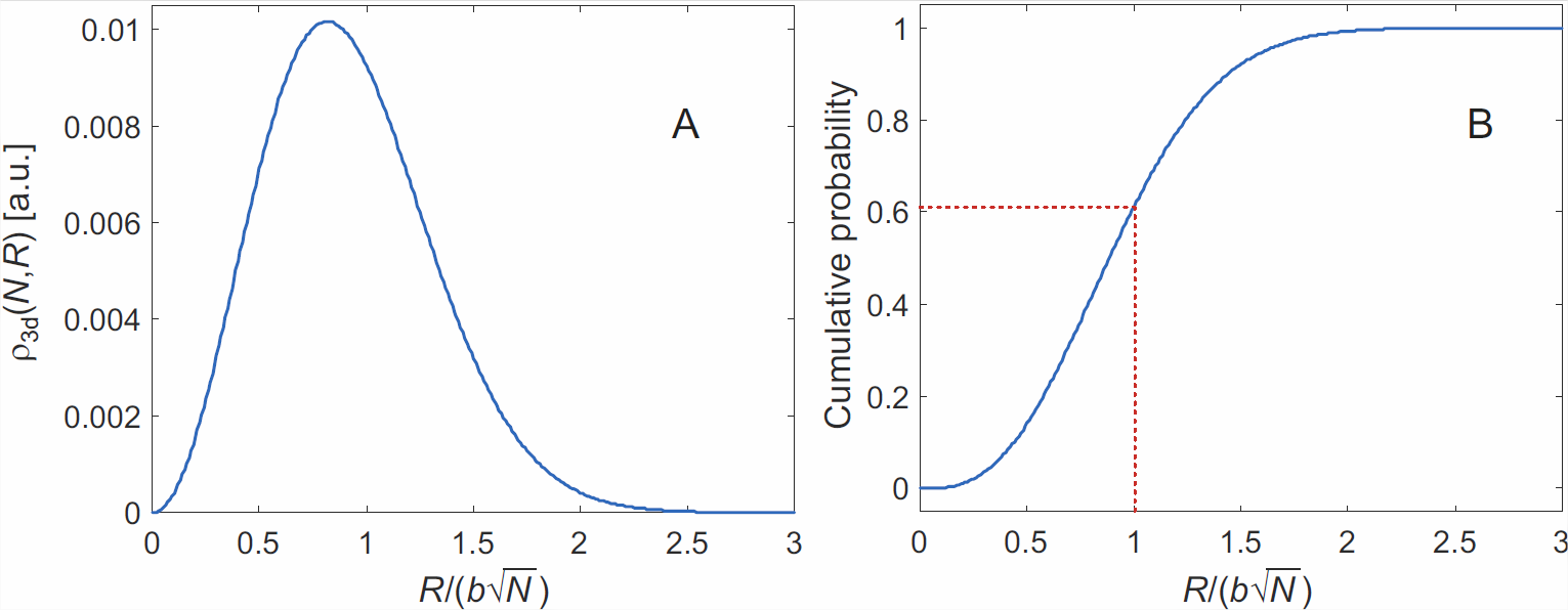
Finally, we can pose the following question: If we let all chains of the ensemble start at the same point, how are the chain ends distributed in space? This is best pictured in a spherical coordinate system. Symmetry dictates that the distribution is uniform with respect to polar angles \(\theta\) and \(\phi\). The polar coordinate \(R\) is equivalent to the end-to-end distance of the chain. To find the probability distribution for this end-to-end distance we need to include area \(4\pi R^2\) of the spherical shells. Hence,

\[\rho_\mathrm{3d}(N,R) \cdot 4 \pi R^2 \mathrm{d} R = 4 \pi \left( \frac{3}{2 \pi N b^2} \right)^{3/2} \exp \left(-\frac{3 R^2}{2 N b^2} \right) R^2 \mathrm{d} R \ .\]

Because of this scaling with the volume of an infinitesimally thin spherical shell, the probability density distribution (Figure \(\PageIndex{1A}\)) for the end-to-end distance does not peak at zero distance. As seen in Figure \(\PageIndex{1B}\) it is very unlikely to encounter a chain with \(R > 2b\sqrt{N}\). Since the contour length is \(R_\mathrm{max} = Nb\), we can conclude that at equilibrium almost all chains have end-to-end distances shorter than \(2 R_\mathrm{max} / \sqrt{N}\).

We need to discuss validity of the result, because in approximating the discrete binomial distribution by a continuous Gaussian probability distribution we had made the assumption \(x \ll N\). Within the ideal chain model, this assumption corresponds to an end-to-end distance that is much shorter than the contour length \(N b\). If \(R\) approaches \(Nb\), the Gaussian distribution overestimates true probability density. In fact, the Gaussian distribution predicts a small, but finite probability for the chain to be longer than its contour length, which is unphysical. The model can be refined to include cases of such strong stretching of the chain . For our qualitative discussion of entropic elasticity not too far from equilibrium, we can be content with Equation \ref{eq:rho3d_chain}).

Conformational Entropy and Free Energy

We may now ask the question of the dependence of free energy on chain extension \(\vec{R}\). With the definition of Boltzmann entropy, Equation \ref{eq:Boltzmann_entropy}), and the usual identification \(k = k_\mathrm{B}\) we have

\[S(N,\vec{R}) = k_\mathrm{B} \ln \Omega(N,\vec{R}) \ .\]

The probability density distribution in Equation \ref{eq:rho3d_chain}) is related to the statistical weight \(\Omega\) by

\[\rho_\mathrm{3d}(N,\vec{R}) = \frac{\Omega(N,\vec{R})}{\int \Omega(N,\vec{R}) \mathrm{d} \vec{R}} \ ,\]

because \(\rho_\mathrm{3d}\) is the fraction of all conformations that have an end-to-end vector in the infinitesimally small interval between \(\vec{R}\) and \(\vec{R} + \mathrm{d}\vec{R}\). Hence,²²

\[\begin{align} S(N,\vec{R}) & = k_\mathrm{B} \ln \rho_\mathrm{3d}(N,\vec{R}) + k_\mathrm{B} \ln \left[ \int \Omega(N,\vec{R}) \mathrm{d} \vec{R} \right] \\ & = -\frac{3}{2} k_\mathrm{B} \frac{\vec{R}^2}{N b^2} + \frac{3}{2} k_\mathrm{B} \ln \left( \frac{3}{2 \pi N b^2} \right) + k_\mathrm{B} \ln \left[ \int \Omega(N,\vec{R}) \mathrm{d} \vec{R} \right] \ . \label{eq:s_N_R_ideal_chain}\end{align}\]

The last two terms do not depend on \(\vec{R}\) and thus constitute an entropy contribution \(S(N,0)\) that is the same for all end-to-end distances, but depends on the number of monomers \(N\),

\[S(N,\vec{R}) = -\frac{3}{2} k_\mathrm{B} \frac{\vec{R}^2}{N b^2} + S(N,0) \ .\]

Since by definition the Kuhn segments of an ideal chain do not interact with each other, the internal energy is independent of \(\vec{R}\). The Helmholtz free energy \(F(N,\vec{R}) = U(N,\vec{R}) - T S(N,\vec{R})\) can thus be written as

\[F(N,\vec{R}) = \frac{3}{2} k_\mathrm{B} T \frac{\vec{R}^2}{N b^2} + F(N,0) \ .\]

It follows that the free energy of an individual chain attains a minimum at zero end-to-end vector, in agreement with our conclusion in Section [subsection:random_walk] that the probability density is maximal for a zero end-to-end vector. At longer end-to-end vectors, chain entropy decreases quadratically with vector length. Hence, the chain can be considered as an entropic spring. Elongation of the spring corresponds to separating the chain ends by a distance \(R \ll N b\). The force required for this elongation is the derivative of Helmholtz free energy with respect to distance. For one dimension, we obtain

\[f_x = -\frac{\partial F\left( N, \vec{R} \right)}{\partial R_x} = -\frac{3 k_\mathrm{B} T}{N b^2} \cdot R_x \ .\]

For the three-dimensional case, the force is a vector that is linear in \(\vec{R}\),

\[\vec{f} = -\frac{3 k_\mathrm{B} T}{N b^2} \cdot \vec{R} \ ,\]

i.e., the entropic spring satisfies Hooke’s law. The entropic spring constant is \(3 k_\mathrm{B} T/(Nb^2)\).

Polymers are thus the easier to stretch the larger their degree of polymerization (proportional to \(N\)), the longer the Kuhn segment \(b\) and the lower the temperature \(T\). In particular, the temperature dependence is counterintuitive. A polymer chain under strain will contract if temperature is raised, since the entropic contribution to Helmholtz free energy, which counteracts the strain, then increases.