
1.1: Basic Assumptions of Statistical Thermodynamics
- Page ID
- 285754
Thermodynamics Based on Statistical Mechanics
Phenomenological thermodynamics describes relations between observable quantities that characterize macroscopic material objects. We know that these objects consist of a large number of small particles, molecules or atoms, and, for all we know, these small particles adhere to the laws of quantum mechanics and often in good approximation to the laws of Newtonian mechanics. Statistical mechanics is the theory that explains macroscopic properties, not only thermodynamic state functions, by applying probability theory to the mechanic equations of motion for a large ensemble of systems of particles. In this lecture course we are concerned with the part of statistical mechanics that relates to phenomenological thermodynamics.
In spite of its name, phenomenological (equilibrium) thermodynamics is essentially a static theory that provides an observational, macroscopic description of matter. The underlying mechanical description is dynamical and microscopic, but it is observational only for systems consisting of a small number of particles. To see this, we consider a system of \(N\) identical classical point particles that adhere to Newton’s equations of motion.
With particle mass \(m\), Cartesian coordinates \(q_i\) \((i = 1, 2, \ldots, 3N)\) and velocity coordinates \(\dot{q}_i\), a system of \(N\) identical classical point particles evolves by
\[\begin{align} & m \frac{\mathrm{d}^2q_i}{\mathrm{d}t^2} = -\frac{\partial}{\partial{q_i}} V\left(q_1, \ldots, q_{3N}\right) \ , \label{eq:Newtonian_eqm}\end{align}\]
where \(V(q_1, \ldots, q_{3N})\) is the potential energy function.
The dynamical state or microstate of the system at any instant is defined by the \(6N\) Cartesian and velocity coordinates, which span the dynamical space of the system. The curve of the system in dynamical space is called a trajectory.
The concept extends easily to atoms with different masses \(m_i\). If we could, at any instant, precisely measure all \(6N\) dynamical coordinates, i.e., spatial coordinates and velocities, we could precisely predict the future trajectory. The system as described by the Newtonian equations of motions behaves deterministically.
For any system that humans can see and handle directly, i.e., without complicated technical devices, the number \(N\) of particles is too large (at least of the order of \(10^{18}\)) for such complete measurements to be possible. Furthermore, for such large systems even tiny measurement errors would make the trajectory prediction useless after a rather short time. In fact, atoms are quantum objects and the measurements are subject to the Heisenberg uncertainty principle, and even the small uncertainty introduced by that would make a deterministic description futile.
We can only hope for a theory that describes what we can observe. The number of observational states or macrostates that can be distinguished by the observer is much smaller than the number of dynamical states. Two classical systems in the same dynamical state are necessarily also in the same observational state, but the converse is not generally true. Furthermore, the observational state also evolves with time, but we have no equations of motion for this state (but see Section [Liouville]). In fact we cannot have deterministic equations of motion for the observational state of an individual system, precisely because the same observational state may correspond to different dynamical states that will follow different trajectories.
Still we can make predictions, only these predictions are necessarily statistical in nature. If we consider a large ensemble of identical systems in the same observational state we can even make fairly precise predictions about the outcome. Penrose gives the example of a women at a time when ultrasound diagnosis can detect pregnancy, but not sex of the fetus. The observational state is pregnancy, the two possible dynamical states are on path to a boy or girl. We have no idea what will happen in the individual case, but if the same diagnosis is performed on a million of women, we know that about 51-52% will give birth to a boy.
How then can we derive stable predictions for an ensemble of systems of molecules? We need to consider probabilities of the outcome and these probabilities will become exact numbers in the limit where the number \(N\) of particles (or molecules) tends to infinity. The theory required for computing such probabilities will be treated in Chapter .
Our current usage of the term ensemble is loose. We will devote the whole Chapter to clarifying what types of ensembles we use in computations and why.
The Markovian Postulate
There are different ways for defining and interpreting probabilities. For abstract discussions and mathematical derivations the most convenient definition is the one of physical or frequentist probability.
Given a reproducible trial \(\mathcal{T}\) of which \(A\) is one of the possible outcomes, the physical probability \(P\) of the outcome \(A\) is defined as
\[\begin{align} & P(A|\mathcal{T}) = \lim\limits_{\mathcal{N} \rightarrow \infty}{\frac{n(A,\mathcal{N},\mathcal{T})}{\mathcal{N}}} \label{eq:phys_prob}\end{align}\]
where \(n(A,\mathcal{N},\mathcal{T})\) is the number of times the outcome \(A\) is observed in the first \(\mathcal{N}\) trials.
A trial \(\mathcal{T}\) conforming to this definition is statistically regular, i.e., the limit exists and is the same for all infinite series of the same trial. If the physical probability is assumed to be a stable property of the system under study, it can be measured with some experimental error. This experimental error has two contributions: (i) the actual error of the measurement of the quantity \(A\) and (ii) the deviation of the experimental frequency of observing \(A\) from the limit defined in Equation \ref{eq:phys_prob}. Contribution (ii) arises from the experimental number of trials \(\mathcal{N}\) not being infinite.
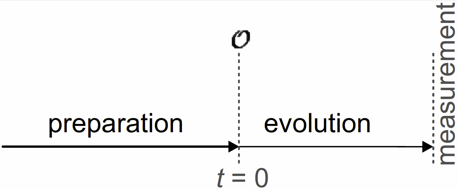
We need some criterion that tells us whether \(\mathcal{T}\) is statistically regular. For this we split the trial into a preparation period, an evolution period, and the observation itself (Figure \(\PageIndex{1}\)). The evolution period is a waiting time during which the system is under controlled conditions. Together with the preparation period it needs to fulfill the Markovian postulate.
A trial \(\mathcal{T}\) that invariably ends up in the observational state \(\mathcal{O}\) of the system after the preparation stage is called statistically regular. The start of the evolution period is assigned a time \(t = 0\).
Note that the system can be in different observational states at the time of observation; otherwise the postulate would correspond to a trivial experiment. The Markovian postulate is related to the concept of a Markovian chain of events. In such a chain the outcome of the next event depends only on the current state of the system, but not on states that were encountered earlier in the chain. Processes that lead to a Markovian chain of events can thus be considered as memoryless.