22.4.4: iv. Problem Solutions

Q1

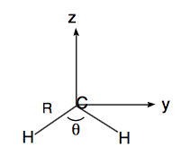
\begin{align} &\text{Molecule I} & & \text{Molecule II}& \\ &R_{CH} = 1.121 Å & & R_{CH} = 1.076 Å & \\ &\angle_{HCH} = 104^{\circ}& & \angle_{HCH} = 136^{\circ} \\ &y_H = \text{ R Sin}\left( \dfrac{\theta}{2} \right) = \pm 0.8834 & & y_H = \pm 0.9976 & \\ &z_H = \text{ R Cos}\left( \dfrac{\theta}{2} \right) = -0.2902 & & z_H = -0.4031 \\ &\text{ Center of Mass(COM):} & & \text{clearly, X = Y = 0, } & \\ & Z = \dfrac{12(0) - 2\text{RCos}\left(\dfrac{\theta}{2}\right)}{14} = -0.0986 & & Z = -0.0576 & \end{align}
a. \begin{align} I_{xx} &=& & \sum\limits_j m_j(y_j^2 + z_j^2) - M(Y^2 + Z^2) \\ T_{xy} &=& & -\sum\limits_j m_jx_jy_j - MXY\end{align}
\begin{align} & I_{xx} = 2(1.121)^2 - 14(-0.0986)^2 & & I_{xx} = 2(1.076)^2 - 14(-0.0576)^2 & \\ & = 2.377 & & = 2.269 & \\ & I_{yy} = 2(0.6902)^2 - 14(-0.0986)^2 & & I_{yy} = 2(0.4031)^2 - 14(-0.0576)^2 & \\ & = 0.8167 & & = 0.2786 & \\ & I_{zz} = 2(0.8834)^2 & & I_{zz} = 2(0.9976)^2 & \\ & =1.561 & & = 1.990 & \\ & I_{xz} = I_{yz} = I_{xy} = 0 & & & \end{align}
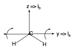
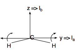
b. Since the moment of inertia tensor is already diagonal, the principal moments of inertia have already been determined to be
\begin{align} & \left( I_a \langle I_b \langle I_c \right): & & &\\ & I_{yy} \langle I_{zz} \langle I_{xx} & & I_{yy} \langle I_{zz} \langle I_{xx} & \\ & 0.8167 \langle 1.561 \langle 2.377 & & 0.2786 \langle 1.990 \langle 2.269 & \end{align}
Using the formula: \( A = \dfrac{h}{8\pi^2cI_a} = \dfrac{6.62x10^{-27}}{8\pi^2(3x10^{10})I_a}\)
\[ A = \dfrac{16.84}{I_a} \text{cm}^{-1} \nonumber \]
similarly, \( B = \dfrac{}{} \text{ cm}^{-1} \text{, and C }= \dfrac{16.84}{I_c} \text{ cm}^{-1}.\)
So,
\begin{align} & \text{Molecule I} & & \text{Molecule II} & \\ & y \Rightarrow A = 20.62 & & y \Rightarrow A = 60.45 & \\ & z \Rightarrow B = 10.79 & & z \Rightarrow B = 8.46 & \\ & x \Rightarrow C = 7.08 & & x \Rightarrow C = 7.42 & \end{align}
c. Averaging B + C:
\begin{align} & B = B \dfrac{B + C}{2} = 8.94 & & B = \dfrac{B + C}{2} = 7.94 & \\ & A - B = 11.68 & & A - B = 52.51 & \end{align}
Using the Prolate top formula
\[ E = (A - B)K^2 + B J(J + 1), \nonumber \]
\begin{align} & \text{Molecule I} & & \text{Molecule II} & \\ & E = 11.68K^2 + 8.94J(J + 1) & & E = 52,51K^2 + 7.94J(J + 1) & \end{align}
Levels: J = 0,1,2,... and K = 0,1, ... J
For a given level defined by J and K, there are \(M_J\) degeneracies given by: (2J + 1)x \begin{Bmatrix} \text{1 for K = 0}\\ \text{2 for K }\ne 0 \end{Bmatrix}
d.

Molecule I		Molecule II

e. Since \(\vec{\mu}\) is along Y, \(\Delta\)K = 0 since K describes rotation about the y axis.
Therefore \(\Delta J = \pm 1\)
f. Assume molecule I is \(CH_2^-\) and molecule II is \(CH_2\). Then, \(\Delta E = E_{J_j}(CH_2)\), where:
\( E(CH_2) = 52.51K^2 + 7.94J(J + 1)\text{, and } E(CH_2) = 11.68K^2 + 8.94J(J + 1) \)
For R-branches: \(J_j = J_i + 1, \Delta K = 0;\)
\begin{align} \Delta E_R &=& &E_{J_j}(CH_2) - E_{J_i}(CH_2) \\ &=& & 7.94(J_i + 1)(J_i + 1 + 1) - 8.94J_i(J_i + 1) \\ &=& & (J_i + 1)\{7.94(J_i + 1 + 1) - 8.94J_i\} \\ &=& &(J_i + 1)\{(7.94 - 8.94)J_i + 2(7.94)\} \\ &=& &(J_i + 1)\{-J_i + 15.88 \} \end{align}
For P-branches: \(J_j - 1, \Delta K = 0;\)
\begin{align} \Delta E_P &=& &E_{J_j}(CH_2) - E_{J_i}(CH_2) \\ &=& & 7.94(J_i - 1)(J_i - 1 + 1) - 8.94J_i(J_i + 1) \\ &=& & J_i \{7.94(J_i - 1) - 8.94(J_i + 1)\} \\ &=& &J_i \{(7.94 - 8.94)J_i - 7.94 - 8.94\} \\ &=& & J_i\{-J_i - 16.88 \} \end{align}

This indicates that the R branch lines occur at energies which grow closer and closer together as J increases (since the 15.88 - \(J_i\) term will cancel). The P branch lines occur at energies which lie more and more negative (i.e. to the left of the origin). So, you can predict that if molecule I is \(CH_2^-\) and molecule II is \(CH_2\) then the R-branch has a band head and the P-branch does not. This is observed therefore our assumption was correct:

molecule I is \(CH_2^-\) and molecule II is \(CH_2\).
g. The band head occurs when \(\dfrac{d(\Delta E_R )}{dJ} = 0\).
\begin{align} \dfrac{d(\Delta E_R)}{dJ} &=& \dfrac{d}{dJ} \left[ (J_i + 1) \{-J_i + 15.88 \} \right] = 0 \\ &=& \dfrac{d}{dJ} \left( -J_i^2 - J_i + 15.88J_i + 15.88 \right) = 0 \\ &=& -2J_i + 14.88 = 0 \\ &\therefore & J_i = 7.44 \text{, so } J = 7 \text{ or } 8. \end{align}

At J = 7.44:
\begin{align} \Delta E_R &=& &(J + 1)\{-J + 15.88\} \\ \Delta E_R &=& &(7.44 + 1)\{ -7.44 + 15.88 \} = (8.44)(8.44) = 71.2 \text{cm}^{-1} \text{above the origin.} \end{align}

Q2

a.

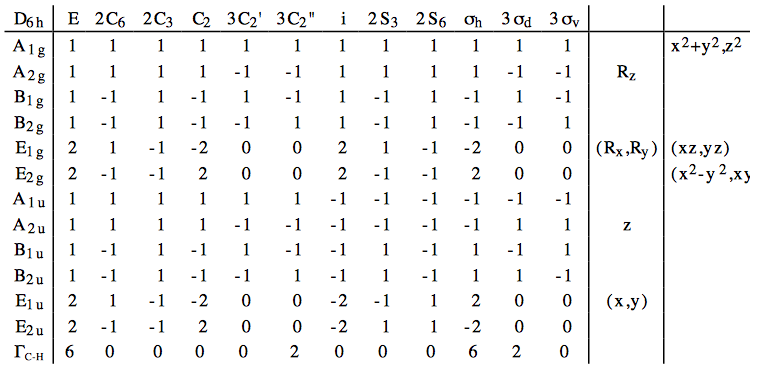
b. The number of irreducible representations may be found by using the following formula:
\begin{align} n_{irrep} &=& &\dfrac{1}{g}\sum\limits_R \xi_{red}(R)\xi_{irrep}(R), \\ \text{where g } &=& & \text{the order of the point group (24 for } D_{6h}). \\ n_{A_{1g}} &=& &\dfrac{1}{24}\sum\limits_R\Gamma_{C-H}(R)\dot{A_{1g}}(R) \\ &=& & \dfrac{1}{24}\{(1)(6)(1) + (2)(0)(1) + (2)(0)(1) + (1)(0)(1) + ... \\ & & & + (3)(0)(1) + (3)(2)(1) + (1)(0)(1) + (2)(0)(1) + ... \\ & & & + (2)(0)(1) + (1)(6)(1) + (3)(2)(1) + (3)(0)(1) \} \\ &=& &1 \\ n_{A_{2g}} &=& & \dfrac{1}{24} \{(1)(6)(1) + (2)(0)(1) + (2)(0)(1) + (1)(0)(1) +... \\ & & & +(3)(0)(-1) + (3)(2)(-1) + (1)(0)(1) + (2)(0)(1) +...\\ & & &+(2)(0)(1) + (1)(6)(1) + (3)(2)(-1) + (3)(0)(-1)\} \\ &=& & 0 \\ n_{B_{1g}} &=& & \dfrac{1}{24} \{(1)(6)(1) + (2)(0)(-1) + (2)(0)(1) + (1)(0)(-1) +... \\ & & & +(3)(0)(1) + (3)(2)(-1) + (1)(0)(1) + (2)(0)(-1) +...\\ & & &+(2)(0)(1) + (1)(6)(-1) + (3)(2)(1) + (3)(0)(-1)\} \\ &=& & 0 \\ n_{B_{2g}} &=& & \dfrac{1}{24} \{(1)(6)(1) + (2)(0)(-1) + (2)(0)(1) + (1)(0)(-1) +... \\ & & & +(3)(0)(-1) + (3)(2)(1) + (1)(0)(1) + (2)(0)(-1) +...\\ & & & + (2)(0)(1) + (1)(6)(-1) + (3)(2)(-1) + (3)(0)(1)\} \\ &=& & 0 \\ n_{E_{1g}} &=& & \dfrac{1}{24} \{(1)(6)(2) + (2)(0)(1) + (2)(0)(-1) + (1)(0)(-2) +... \\ & & & +(3)(0)(0) + (3)(2)(0) + (1)(0)(2) + (2)(0)(1) +...\\ & & &+(2)(0)(-1) + (1)(6)(-2) + (3)(2)(0) + (3)(0)(0)\} \\ &=& & 0 \\ n_{E_{2g}} &=& & \dfrac{1}{24} \{(1)(6)(2) + (2)(0)(-1) + (2)(0)(-1) + (1)(0)(2) +... \\ & & & +(3)(0)(0) + (3)(2)(0) + (1)(0)(2) + (2)(0)(-1) +...\\ & & &+(2)(0)(-1) + (1)(6)(2) + (3)(2)(0) + (3)(0)(0)\} \\ &=& & 0 \\ n_{A_{1u}} &=& & \dfrac{1}{24} \{(1)(6)(1) + (2)(0)(1) + (2)(0)(1) + (1)(0)(1) +... \\ & & & +(3)(0)(1) + (3)(2)(1) + (1)(0)(-1) + (2)(0)(-1) +...\\ & & & + (2)(0)(-1) + (1)(6)(-1) + (3)(2)(-1) + (3)(0)(-1)\} \\ &=& & 0 \\ n_{A_{2u}} &=& & \dfrac{1}{24} \{(1)(6)(1) + (2)(0)(1) + (2)(0)(1) + (1)(0)(1) +... \\ & & & + (3)(0)(-1) + (3)(2)(-1) + (1)(0)(-1) + (2)(0)(-1) +...\\ & & &+(2)(0)(-1) + (1)(6)(-1) + (3)(2)(1) + (3)(0)(1)\} \\ &=& & 0 \\ n_{B_{1u}} &=& & \dfrac{1}{24} \{(1)(6)(1) + (2)(0)(-1) + (2)(0)(1) + (1)(0)(-1) +... \\ & & & +(3)(0)(1) + (3)(2)(-1) + (1)(0)(-1) + (2)(0)(1) +...\\ & & & + (2)(0)(-1) + (1)(6)(1) + (3)(2)(-1) + (3)(0)(1)\} \\ &=& & 0 \\ n_{B_{2u}} &=& & \dfrac{1}{24} \{(1)(6)(1) + (2)(0)(-1) + (2)(0)(1) + (1)(0)(-1) +... \\ & & & +(3)(0)(-1) + (3)(2)(1) + (1)(0)(-1) + (2)(0)(1) +...\\ & & &+(2)(0)(-1) + (1)(6)(1) + (3)(2)(1) + (3)(0)(-1)\} \\ &=& & 1 \\ n_{E_{1u}} &=& & \dfrac{1}{24} \{(1)(6)(2) + (2)(0)(1) + (2)(0)(-1) + (1)(0)(-2) +... \\ & & & +(3)(0)(0) + (3)(2)(0) + (1)(0)(-2) + (2)(0)(-1) +...\\ & & &+(2)(0)(1) + (1)(6)(2) + (3)(2)(0) + (3)(0)(0)\} \\ &=& & 1 \\n_{E_{2u}} &=& & \dfrac{1}{24} \{(1)(6)(2) + (2)(0)(-1) + (2)(0)(-1) + (1)(0)(2) +... \\ & & & +(3)(0)(0) + (3)(2)(0) + (1)(0)(-2) + (2)(0)(1) +...\\ & & & + (2)(0)(1) + (1)(6)(-2) + (3)(2)(0) + (3)(0)(0)\} \\ &=& & 0 \end{align}
We see that \(\Gamma_{C-H} = A_{1g}\oplus E_{2g}\oplus B_{2u}\oplus E_{1u}\)

c. x and y \(\Rightarrow\) \(E_{1u} \text{, z } \Rightarrow A_{2u}\), so, the ground state \(A_{1g}\) level can be excited to the degenerate \(E_{1u}\) level by coupling through the x or y transition dipoles. Therefore \(E_{1u}\) is infrared active and \(\perp\) polarized.

d. \( (x^2 + y^2, z^2 ) \Rightarrow A_{1g}, (xz, yz) \Rightarrow E_{1g}, (x^2 - y^2, xy) \Rightarrow E_{2g}\), so, the ground sate \(A_{1g}\) level can be excited to the degenerate \(E_{2g}\) level by coupling through the \(x^2 - y^2 \) or xy transitions or be excited to the degenerate \(A_{1g}\) level by coupling through the xz or yz transitions. Therefore \(A_{1g} \text{ and } E_{2g}\) are Raman active.

Q3

a.
\begin{align} \dfrac{d}{dr}\left( \dfrac{F}{r} \right) &=& & \dfrac{F'}{r} - \dfrac{F}{r^2} \\ r^2 \dfrac{d}{dr} \left( \dfrac{F}{r} \right) &=& & rF' - F \\ \dfrac{d}{dr} \left( r^2 \dfrac{d}{dr} \left( \dfrac{F}{r} \right) \right) &=& & F' - F' + rF'' \end{align}
So,
\begin{align} \dfrac{-\hbar^2}{2\mu r^2}\dfrac{d}{dr}\left( r^2 \dfrac{d}{dr}\left( \dfrac{F}{r} \right) \right) &=& & \dfrac{-\hbar^2}{2\mu} \dfrac{F''}{r}\end{align}
Rewriting the radial Schrödinger equation with the substitution: \( R = \dfrac{F}{r}\) gives:
\[ \dfrac{-h^2}{2\mu r^2}\dfrac{d}{dr} \left( r^2 \dfrac{d(Fr^{-1})}{dr} \right) + \dfrac{J(J + 1)\hbar^2}{2\mu r^2} \left(\dfrac{F}{r}\right) + \dfrac{1}{2} k(r - r_e)^2 \left( \dfrac{F}{r} \right) = \left( \dfrac{F}{r} \right) \nonumber \]
Using the above derived identity gives:
\[ \dfrac{-\hbar^2}{2\mu}\dfrac{F''}{r} + \dfrac{J(J + 1)\hbar^2}{2\mu r^2} \left( \dfrac{F}{r} \right) + \dfrac{1}{2}k(r - r_e)^2 \left( \dfrac{F}{r} \right) = E \left( \dfrac{F}{r} \right) \nonumber \]
Cancelling out an \(r^{-1}\):
\[ \dfrac{-\hbar^2}{2\mu} F'' + \dfrac{J(J + 1)\hbar^2}{2\mu r^2}F + \dfrac{1}{2} k(r - r_e)^2 F = EF \nonumber \]

b. \[ \dfrac{1}{r^2} = \dfrac{1}{(r_e + \Delta r)^2} = \dfrac{1}{r_e^2 \left( 1 + \dfrac{\Delta r}{r_e} \right)} \approx \dfrac{1}{r_e^2}\left( 1 - \dfrac{2\Delta r}{r_e} + \dfrac{3\Delta r^2}{r_e^2} \right) \nonumber \]
So,
\[ \dfrac{J(J + 1)\hbar^2}{2\mu r^2} \approx \dfrac{J(J + 1)\hbar^2}{2\mu r_e^2}\left( 1 - \dfrac{2\Delta r}{r_e} + \dfrac{3\Delta r^2}{r_e^2} \right) \nonumber \]

c. Using this substitution we now have:
\[ \dfrac{-\hbar^2}{2\mu} F'' + \dfrac{J(J + 1)\hbar^2}{2\mu r_e^2} \left( 1 - \dfrac{2\Delta r}{r_e} + \dfrac{3\Delta r^2}{r_e^2} \right) F + \dfrac{1}{2} k(r - r_e)^2 F = EF \nonumber \]
Now, regroup the terms which are linear and quadratic in \(\Delta r = r - r_e\):
\[ \dfrac{1}{2} k\Delta r^2 + \dfrac{J(J + 1)\hbar^2}{2\mu r_e^2}\dfrac{3}{r_e^2}\Delta r^2 - \dfrac{J(J + 1)\hbar^2}{2\mu r_e^2}\dfrac{2}{r_e}\Delta r \nonumber \]
\[ = \left( \dfrac{1}{2}k + \dfrac{J(J + 1)\hbar^2}{2\mu r_e^2}\dfrac{3}{r_e^2} \right) \Delta r^2 - \left( \dfrac{J(J + 1)\hbar^2}{2\mu r_e^2} \dfrac{2}{r_e} \right)\Delta r \nonumber \]
Now, we must complete the square:
\[ a\Delta r^2 - b\Delta r = a \left( \Delta r - \dfrac{b}{2a} \right)^2 - \dfrac{b^2}{4a}. \nonumber \]
So,
\[ \left( \dfrac{1}{2}k + \dfrac{J(J + 1)\hbar^2}{2\mu r_e^2}\dfrac{3}{r_e^2} \right)\left( \Delta r - \dfrac{\dfrac{J(J + 1)\hbar^2}{2\mu r_e^2}\dfrac{1}{r_e}}{\dfrac{1}{2}k + \dfrac{J(J + 1)\hbar^2}{2\mu r_e^2}\dfrac{3}{r_e^2}} \right)^2 - \dfrac{\left( \dfrac{J(J + 1)\hbar^2}{2\mu r_e^2} \dfrac{1}{r_e} \right)^2}{\dfrac{1}{2}k + \dfrac{J(J + 1)\hbar^2}{2\mu r_e^2}\dfrac{3}{r_e^2}} \nonumber \]
Now, redefine the first term as \(\dfrac{1}{2}k\), second term as (r - \(\bar{r_e})^2\), and the third term as \(-\Delta \) giving:
\[ \dfrac{1}{2}\bar{k} \left(r - \bar{r_e}\right)^2 - \Delta \nonumber \]
From:
\begin{align} & & &\dfrac{-\hbar^2}{2\mu}F'' + \dfrac{J(J + 1)\hbar^2}{2\mu r_e^2} \left( 1 - \dfrac{2\Delta r}{r_e} + \dfrac{3\Delta r^2}{r_e^2} \right) F + \dfrac{1}{2} k(r - r_e)^2 F = EF, \\ & & & \dfrac{-\hbar^2}{2\mu} F'' + \dfrac{J(J + 1)\hbar^2}{2\mu r_e} F + \left( \dfrac{J(J + 1)\hbar^2}{2\mu r_e^2} \left( - \dfrac{2\Delta r}{r_e} + \dfrac{3\Delta r^2}{r_e^2} \right) + \dfrac{1}{2}k\Delta r^2 \right) F = EF \end{align}
and making the above substitution result in:
\[ \dfrac{-\hbar^2}{2\mu}F'' + \dfrac{J(J + 1)\hbar^2}{2\mu r_e^2}F + \left( \dfrac{1}{2}\bar{k} \left( r - \bar{r_e}\right)^2 - \Delta \right) F = EF, \nonumber \]
or,
\[ \dfrac{-\hbar^2}{2\mu}F'' + \dfrac{1}{2}\bar{k} (r - r\bar{r_e} )^2 F = \left( E - \dfrac{J(J + 1)\hbar^2}{2\mu r_e^2} + \Delta \right) F. \nonumber \]

d. Since the above is nothing but a harmonic oscillator differential equation in x with force constant \(\bar{k}\) and equilibrium bond length \(\bar{r}_e\), we know that:
\begin{align} & & &\dfrac{-\hbar^2}{2\mu}F'' + \dfrac{1}{2} \bar{k} (r - \bar{r}_e)^2 F \varepsilon F\text{, has energy levels:} \\ & & & \varepsilon = \hbar \sqrt{\dfrac{\bar{k}}{\mu}}\left(v + \dfrac{1}{2}\right) \text{, v = 0, 1, 2, ... } \end{align}
So,
\begin{align} & & & E + \Delta . - \dfrac{J(J + 1)\hbar^2}{2\mu r_e^2} = \varepsilon \end{align}
tell us that:
\begin{align} & & & E = \hbar\sqrt{\dfrac{\bar{k}}{\mu}}\left( v + \dfrac{1}{2} \right) + \dfrac{J(J + 1)\hbar^2}{2\mu r_e^2} - \Delta .\end{align}
As J increases, \(\bar{r}_e\) increases because of the centrifugal force pushing the two atoms apart. On the other hand \(\bar{k}\) increases which inicates that the molecule finds it more difficult to stretch against both the centrifugal and Hooke's Law (spring) Harmonic force field. The total energy level (labeled by J and v) will equal a rigid rotor componenet \(\dfrac{J(J + 1)\hbar^2}{2\mu r_e^2}\) plus a Harmonic oscillator part \(\hbar \sqrt{\dfrac{\bar{k}}{\mu}\left( v + \dfrac{1}{2}\right)}\) (which has a force constant \(\bar{k}\) which increases with J).