
16.1: One Dimensional Scattering
- Page ID
- 60582

Atom-atom scattering on a single Born-Oppenheimer energy surface can be reduced to a one-dimensional Schrödinger equation by separating the radial and angular parts of the three-dimensional Schrödinger equation in the same fashion as used for the Hydrogen atom in Chapter 1. The resultant equation for the radial part \(\psi\)(R) of the wavefunction can be written as:
\[ -\left( \dfrac{\hbar^2}{2\mu} \right) \dfrac{1}{R^2} \dfrac{\partial }{\partial R} \left( R^2\dfrac{\partial \psi}{\partial R} \right) + L(L+1)\dfrac{\hbar^2}{(2\mu R^2)} \psi + V(R)\psi = E\psi , \nonumber \]
where L is the quantum number that labels the angular momentum of the colliding particles whose reduced mass is \(\mu\).
Defining \(\Psi(R) = R \psi(R)\text{ and substituting into the above equation gives the following equation for } \Psi :\)
\[ \left( \dfrac{\hbar^2}{2\mu} \right) \dfrac{\partial^2\Psi}{\partial R^2} + L(L+1)\dfrac{\hbar^2}{2\mu R^2}\Psi + V(R)\Psi = E\Psi . \nonumber \]
The combination of the "centrifugal potential" \( L(L+1)\frac{\hbar^2}{2\mu R^2} \) and the electronic potential V(R) thus produce a total "effective potential" for describing the radial motion of the system.
The simplest reasonable model for such an effective potential is provided by the "square well" potential illustrated below. This model V(R) could, for example, be applied to the L = 0 scattering of two atoms whose bond dissociation energy is \(D_e\) and whose equilibrium bond length for this electronic surface lies somewhere between R = 0 and R = \(\text{R}_{\text{max}}\).
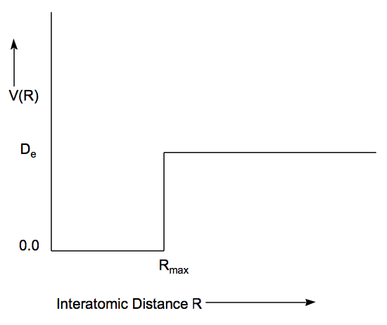
The piecewise constant nature of this particular V(R) allows exact solutions to be written both for bound and scattering states because the Schrödinger equation
\[ -\left( \dfrac{\hbar^2}{2\mu} \right) \dfrac{\text{d}^2\Psi}{\text{d}R^2} = E\Psi \text{ ( for 0 } \leq \text{ R } \leq \text{R}_{\text{max}}) \nonumber \]
\[ -\left( \dfrac{\hbar^2}{2\mu} \right) \dfrac{\text{d}^2\Psi}{\text{d}R^2} + D_e\Psi = E \Psi \text{ R}_{\text{max}} \leq \text{ R } < \infty ) \nonumber \]
admits simple sinusoidal solutions.
Bound States
The bound states are characterized by having E < D\(_e\). For the inner region, the two solutions to the above equation are
\[ \Psi_1(R) = A sin(kR) \nonumber \]
and
\[ \Psi_2(R) = B cos(kR) \nonumber \]
where
\[ k = \sqrt{\dfrac{2\mu E}{\hbar^2}} \nonumber \]
is termed the "local wave number" because it is related to the momentum values for the \(e^{\pm ikR}\) components of such a function:
\[ \dfrac{-i\hbar \partial e^{\pm ikR}}{\partial R} = \hbar k e^{\pm ikR}. \nonumber \]
The cos(kR) solution must be excluded (i.e., its amplitude B in the general solution of the Schrödinger equation must be chosen equal to 0.0) because this function does not vanish at R = 0, where the potential moves to infinity and thus the wavefunction must vanish. This means that only the
\[ \Psi = A sin(kR) \nonumber \]
term remains for this inner region.
Within the asymptotic region (R > R\(_{max}\)) there are also two solutions to the Schrödinger equation:
\[ \Psi_3 = Ce^{-\kappa R} \nonumber \]
and
\[ \Psi_4 = D e^{\kappa R} \nonumber \]
where
\[ \kappa = \sqrt{\dfrac{2\mu (D_e-E)}{\hbar^2}}. \nonumber \]
Clearly, one of these functions is a decaying function of R for large R and the other \(\Psi_4\) grows exponentially for large R. The latter's amplitude D must be set to zero because this function generates a probability density that grows larger and larger as R penetrates deeper and deeper into the classically forbidden region (where E < V(R)).
To connect \(\Psi_1\) in the inner region to \(\Psi_3\) in the outer region, we use the fact that \(\Psi\) and \(\frac{\text{d} \Psi}{\text{dR}}\) must be continuous except at points R where V(R) undergoes an infinite discontinuity (see Chapter 1). Continuity of \(\Psi \text{at R}_{max}\) gives:
\[ \text{Asin}(\text{kR}_{max}) = Ce^{-\kappa\text{R}_{\text{max}}}, \nonumber \]
and continuity of \( \frac{\text{d}\Psi}{\text{dR}} \text{at R}_{\text{max}} \) yields
\[ Akcos(kR_{max})= - \kappa C e^{-\kappa R_{max}} \nonumber \]
These two equations allow the ratio C/A as well as the energy E (which appears in \(\kappa\) and in k) to be determined:
\[ \dfrac{A}{C} = \dfrac{-\kappa}{k}\dfrac{e^{-\kappa R_{max}}}{cos(kR_{max})}. \nonumber \]
The condition that determines E is based on the well known requirement that the determinant of coefficients must vanish for homogeneous linear equations to have no-trivial solutions (i.e., not A = C = 0):
\[ \det\left( \matrix{sin(kR_{max}) & -e^{-\kappa R_{max}} \cr kcos(kR_{max}) & \kappa e^{-\kappa R_{max}}}\right) = 0 \nonumber \]
The vanishing of this determinant can be rewritten as
\[ \kappa sin(kR_{max}) e^{-\kappa R_{max}} + kcos(kR_{max})e^{-\kappa R_{max}} = 0 \nonumber \]
or
\[ tan(kR_{max}) = \dfrac{-\kappa}{k}. \nonumber \]
When employed in the expression for A/C, this result gives
\[ \dfrac{A}{C} = \dfrac{e^{-\kappa R_{max}}}{sin(kR_{max})} \nonumber \]
For very large D\(_e\) compared to E, the above equation for E reduces to the familiar "particle in a box" energy level result since \(\frac{k}{\kappa}\) vanishes in this limit, and thus tan(kR\(_{max}\)) = 0, which is equivalent to sin(kR\(_{max}\)) = 0, which yields the familiar \( \text{E} = \frac{n^2h^2}{8\mu R^2_{\text{max}}} \) and \(\frac{C}{A}\) = 0, so \(\Psi = \text{ A sin}(\text{kR}\)).
When D\(_e\) is not large compared to E, the full transcendental equation \(\text{tan(kR}_{\text{max}}) = -\frac{k}{\kappa}\) must be solved numerically or graphically for the eigenvalues \(\text{E}_n\), n = 1, 2, 3, ... . These energy levels, when substituted into the definitions for k and \(\kappa\) give the wavefunctions:
\[ \Psi = \text{A sin(kR) (for 0} \leq \text{ R } \leq \text{ R}_{\text{max}}) \nonumber \]
\[ \Psi = \text{A sin(kR}_{\text{max}})e^{\kappa \text{R}_{\text{max}}}e^{-\kappa R}\text{ (for R}_{\text{max}} \leq \text{R < }\infty). \nonumber \]
The one remaining unknown A can be determined by requiring that the modulus squared of the wavefunction describe a probability density that is normalized to unity when integrated over all space:
\[ \int\limits_{0}^{\infty}|\Psi |^2 \text{dR} = 1. \nonumber \]
Note that this condition is equivalent to
\[ \int\limits_{0}^{\infty} |\Psi |^2 \text{R}^2\text{dR} = 1 \nonumber \]
which would pertain to the original radial wavefunction. In the case of an infinitely deep potential well, this normalization condition reduces to
\[ \int\limits_{0}^{\text{R}_{\text{max}}}\text{A}^2\text{sin}^2\text{(kR)}\text{dR} = 1 \nonumber \]
which produces
\[ \text{A} = \sqrt{\dfrac{2}{\text{R}_{\text{max}}} }. \nonumber \]
Scattering States
The scattering states are treated in much the same manner. The functions \(\Psi_1 \text{ and } \Psi_2 \text{ arise as above, and the amplitude of } \Psi_2 \text{ must again be chosen to vanish because } \Psi\) must vanish at R = 0 where the potential moves to infinity. However, in the exterior region (R> R\(_{\text{max}}\)), the two solutions are now written as:
\[ \Psi_3 = Ce^{\text{ik'R}} \nonumber \]
\[ \Psi_4 = De^{-\text{ik'R}} \nonumber \]
where the large-R local wavenumber
\[ k' = \sqrt{\dfrac{2\mu (E-D_e)}{\hbar^2}} \nonumber \]
arises because E > \(\text{D}_e\) for scattering states.
The conditions that \(\Psi \text{ and } \frac{\text{d}\Psi}{\text{dR}} \text{ be continuous at R}_{\text{max}}\) still apply:
\[ \text{Asin(kR}_{\text{max}}) = Ce^{\text{ik'R}_{\text{max}}}-\text{ik'D}e^{\text{-ik'R}_{\text{max}}}. \nonumber \]
and
\[ \text{kAcos(kR}_{\text{max}}) = \text{ik'C}e^{\text{ik'R}_{\text{max}}}-\text{ik'D}e^{\text{-ik'R}_{\text{max}}}. \nonumber \]
However, these two equations (in three unknowns A, C, and D) can no longer be solved to generate eigenvalues E and amplitude ratios. There are now three amplitudes as well as the E value but only these two equations plus a normalization condition to be used. The result is that the energy no longer is specified by a boundary condition; it can take on any value. We thus speak of scattering states as being "in the continuum" because the allowed values of E form a continuum beginning at E = \(\text{D}_e\) (since the zero of energy is defined in this example as at the bottom of the potential well).
The R > R\(_\text{max}\) components of \(\Psi\) are commonly referred to as "incoming"
\[ \Psi_{\text{in}} = \text{D}e^{\text{-ik'R}} \nonumber \]
and "outgoing"
\[ \Psi_{\text{out}} = Ce^{\text{ik'R}} \nonumber \]
because their radial momentum eigenvalues are -\(\hbar \text{ k' and } \hbar\) k', respectively. It is a common convention to define the amplitude D so that the flux of incoming particles is unity.
Choosing
\[ \text{D} = \sqrt{\dfrac{\mu}{\hbar k'}} \nonumber \]
produces an incoming wavefunction whose current density is:
\[ \text{S(R) = } \dfrac{-i\hbar}{2\mu}\left[ \Psi^{\text{*}}_{\text{in}}\left( \dfrac{\text{d}}{\text{dR}\Psi_{\text{in}}} \right) - \left( \dfrac{\text{d}\Psi_{\text{in}}}{\text{dR}} \right)^{\text{*}}\Psi_{\text{in}} \right] \nonumber \]
\[ = |\text{D}|^2 \left( \dfrac{-i\hbar}{2\mu} \right) [-2ik'] \nonumber \]
\[ = -1. \nonumber \]
This means that there is one unit of current density moving inward (this produces the minus sign) for all values of R at which \(\Psi_{\text{in}}\) is an appropriate wavefunction (i.e., R > \(\text{R}_{\text{max}}\)). This condition takes the place of the probability normalization condition specified in the boundstate case when the modulus squared of the total wavefunction is required to be normalized to unity over all space. Scattering wavefunctions can not be so normalized because they do not decay at large R; for this reason, the flux normalization condition is usually employed. The magnitudes of the outgoing (C) and short range (A) wavefunctions relative to that of the incoming function (D) then provide information about the scattering and "trapping" of incident flux by the interaction potential.
Once D is so specified, the above two boundary matching equations are written as a set of two inhomogeneous linear equations in two unknowns (A and C):
\[ \text{Asin(kR}_{\text{max}}) - Ce^{\text{ik'R}_{\text{max}}} = De^{\text{-ik'R}_{\text{max}}}) \nonumber \]
and
\[ \text{kAcos(kR}_{\text{max}}) - \text{ik'C}e^{\text{ik'R}_{\text{max}}}) = \text{-ik'D}e^{\text{-ik'R}_{\text{max}}} \nonumber \]
or
\[ \left( \matrix{ \text{sin(kR}_{\text{max}}) & -e^{\text{ik'R}_{\text{max}}} \cr \text{kcos(kR}_{\text{max})} & \text{-ik'}e^{\text{ik'R}_{\text{max}}} } \right) \left( \matrix{A \cr C} \right) = \left( \matrix{ \text{D}e^{\text{-ik'R}_{\text{max}}} \cr \text{-ik'D}e^{\text{-ik'R}_{\text{max}}} } \right). \nonumber \]
Non-trivial solutions for A and C will exist except when the determinant of the matrix on the left side vanishes:
\[ \text{-ik'sin(kR}_{\text{max}}) + \text{kcos(kR}_{\text{max}}) = 0, \nonumber \]
which can be true only if
\[ \text{tan(kR}_{\text{max}}) = \dfrac{\text{ik'}}{\text{k}}. \nonumber \]
This equation is not obeyed for any (real) value of the energy E, so solutions for A and C in terms of the specified D can always be found.
In summary, specification of unit incident flux is made by choosing D as indicated above. For any collision energy E > D\(_e\), the 2x1 array on the right hand side of the set of linear equations written above can be formed, as can the 2x2 matrix on the left side. These linear equations can then be solved for A and C. The overall wavefunction for this E is then given by:
\[ \matrix{\Psi = \text{Asin(kR)} & \text{(for 0 } \leq \text{ R } \leq \text{ R}_{\text{max}}) \cr \Psi =Ce^{\text{ik'R}} + De^{\text{-ik'R}} & \text{(for R}_{\text{max}} \leq \text{R} < \infty). } \nonumber \]
Shape Resonance States
If the angular momentum quantum number L in the effective potential introduced earlier is non-zero, this potential has a repulsive component at large R. This repulsion can combine with short-range attractive interactions due, for example, to chemical bond forces, to produce an effective potential that one can model in terms of simple piecewise functions shown below.
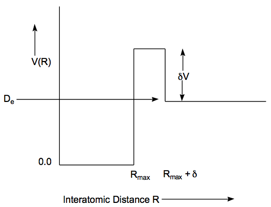
Again, the piecewise nature of the potential allows the one-dimensional Schrödinger equation to be solved analytically. For energies below D\(_e\), one again finds bound states in much the same way as illustrated above (but with the exponentially decaying function \(e^{\text{-k'R}} \text{ used in the region } \text{R}_\text{max} \leq \text{R} \leq \text{R}_{\text{max}} + \delta\text{, with } \kappa ' = \sqrt{2\mu(-D_e-\delta V - E)/\hbar^2}). \)
For energies lying above D\(_e\) + \(\delta\)V, scattering states occur and the four amplitudes of the functions (sin(kR), e\(^{\text{(±i k'''R)}} \text{ with k''' = } \sqrt{2\mu(D_e + \delta V + E)/\hbar^2}), \text{ and e}^{\text{(ik'R)}})\) appropriate to each R-region are determined in terms of the amplitude of the incoming asymptotic function \( \text{De}^{\text{(-ik'R)}} \text{ from the four equations obtained by matching } \Psi \text{ and } \frac{\text{d}\Psi}{\text{dR}} \text{ at R}_{\text{max}} \text{ and at } \text{R}_{\text{max}} + \delta\).
For energies lying in the range D\(_e\) < E < D\(_e \text{ + }\delta V\), a qualitatively different class of scattering function exists. These so-called shape resonance states occur at energies that are determined by the condition that the amplitude of the wavefunction within the barrier (i.e., for 0 \(\leq \text{ R } \leq \text{R}_{\text{max}}\) ) be large so that incident flux successfully tunnels through the barrier and builds up, through constructive interference, large probability amplitude there. Let us now turn our attention to this specific energy regime.
The piecewise solutions to the Schrödinger equation appropriate to the shaperesonance case are easily written down:
\[ \matrix{ & \Psi = \text{Asin(kR)} & \text{(for 0 } \leq \text{ R } \leq \text{R}_{\text{max}}) \cr & \Psi = \text{B}_+e^{\kappa '\text{R}} + \text{B}_-e^{-\kappa '\text{R}} & \text{(for R}_{max} \leq \text{ R } \leq \text{R}_{\text{max}} + \delta ) \cr & \Psi = \text{C}e^{\text{ik'R}} + \text{D}e^{\text{-ikR}} & \text{(for R}_{\text{max}} + \delta \leq \text{ R } \leq \infty) } \nonumber \]
Note that both exponentially growing and decaying functions are acceptable in the \(R_{max} \leq \text{ R } \leq \text{R}_{\text{max}} +\delta\) region because this region does not extend to \(\text{R} = \infty\). There are four amplitudes (A, B+, B- , and C) that must be expressed in terms of the specified amplitude D of the incoming flux. Four equations that can be used to achieve this goal result when \(\Psi \text{ and } \frac{\text{d}\Psi}{\text{dR}} \text{ are matched at R}_{max} \text{ and at R}_{max} + \delta\):
\[ \matrix{ & Asin(kR_{max}) = B_+e^{\kappa 'R_{max}} + B_-e^{-\kappa 'R_{max}}, \cr & Akcos(kR_{max}) = \kappa 'B_+e^{\kappa 'R_{max}} -\kappa 'B_-e^{-\kappa 'R_{max}}, \cr & B_+e^{\kappa '(R_{max}+\delta)} +B_-e^{-\kappa '(R_{max}+\delta)} = Ce^{ik'(R_{max} + \delta)} + De^{-ik'(R_{max} + \delta)}, \cr & \kappa 'B_+e^{\kappa '(R_{max} + \delta)} -\kappa 'B_-e^{-\kappa '(R_{max} + \delta)} \cr & = ik'Ce^{ik'(R_{max} + \delta)} -ik'De^{ik'(R_{max}+\delta)}. } \nonumber \]
It is especially instructive to consider the value of A/D that results from solving this set of four equations in four unknowns because the modulus of this ratio provides information about the relative amount of amplitude that exists inside the centrifugal barrier in the attractive region of the potential compared to that existing in the asymptotic region as incoming flux.
The result of solving for A/D is:
\[ \dfrac{A}{D} = \dfrac{4\kappa 'e^{-ik'(R_{max}+\delta)}}{\left[ \dfrac{e^{\kappa '\delta}(ik'-\kappa ')(\kappa 'sin(kR_{max})+kcos(kR_{max}))}{ik'} + \dfrac{e^{- \kappa '\delta}(ik'+\kappa ')(\kappa 'sin(kR_{max})-kcos(kR_{max}))}{ik'} \right]^{-1}} \nonumber \]
Further, it is instructive to consider this result under conditions of a high (large \(D_e + \delta\)V - E) and thick (large \(\delta\)) barrier. In such a case, the "tunnelling factor" \( e^{-\kappa '\delta}\) will be very small compared to its counterpart \( e^{\kappa '\delta} \), and so
\[ \dfrac{A}{D} = 4\dfrac{ik'\kappa '}{ik'-\kappa '}e^{-ik'(R_{max}+\delta)}\dfrac{e^{-\kappa '\delta}}{\kappa 'sin(kR_{max})+kcos(kR_{max})}. \nonumber \]
The \(e^{-\kappa '\delta}\) factor in A/D causes the magnitude of the wavefunction inside the barrier to be small in most circumstances; we say that incident flux must tunnel through the barrier to reach the inner region and that \( e^{-\kappa '\delta} \) gives the probability of this tunnelling. The magnitude of the A/D factor could become large if the collision energy E is such that
\[ \kappa 'sin(kR_{max})+kcos(kR_{max}) \nonumber \]
is small. In fact, if
\[ tan(kR_{max}) = \dfrac{-k}{\kappa '} \nonumber \]
this denominator factor in A/D will vanish and A/D will become infinite. Note that the above condition is similar to the energy quantization condition
\[ tan(kR_{max}) = \dfrac{-k}{\kappa} \nonumber \]
that arose when bound states of a finite potential well were examined earlier in this Chapter. There is, however, an important difference. In the bound-state situation
\[ k = \sqrt{\dfrac{2\mu E}{\hbar^2}} \nonumber \]
and
\[ \kappa = \sqrt{\dfrac{2\mu (D_e - E)}{\hbar^2}}; \nonumber \]
in this shape-resonance case, k is the same, but
\[ \kappa ' = \sqrt{\dfrac{2\mu (D_e + \delta V - E)}{\hbar^2}} \nonumber \]
rather than \(\kappa\) occurs, so the two tan(k\(R_{max}\)) equations are not identical.
However, in the case of a very high barrier (so thats \(\kappa '\) is much larger than k), the denominator
\[ \kappa ' sin(kR_{max}) + kcos(kR_{max}) \approx \kappa 'sin(kR_{max}) \nonumber \]
in A/D can become small if
\[ sin(kR_{max}) \approx 0. \nonumber \]
This condition is nothing but the energy quantization condition that would occur for the particle-in-a-box potential shown below.
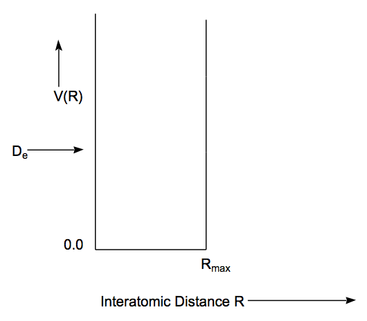
This potential is identical to the true effective potential for \(0 \leq R \leq R_{max}\), but extends to infinity beyond \(R_{max}\) ; the barrier and the dissociation asymptote displayed by the true potential are absent.
In summary, when a barrier is present on a potential energy surface, at energies above the dissociation asymptote \(D_e\) but below the top of the barrier \((D_e + \delta V\) here), one can expect shape-resonance states to occur at "special" scattering energies E. These socalled resonance energies can often be approximated by the bound-state energies of a potential that is identical to the potential of interest in the inner region \((0 \leq R \leq R_{max}\) here) but that extends to infinity beyond the top of the barrier (i.e., beyond the barrier, it does not fall back to values below E).
The chemical significance of shape resonances is great. Highly rotationally excited molecules may have more than enough total energy to dissociate \((D_e)\), but this energy may be "stored" in the rotational motion, and the vibrational energy may be less than \(D_e\). In terms of the above model, high angular momentum may produce a significant barrier in the effective potential, but the system's vibrational energy may lie significantly below \(D_e\). In such a case, and when viewed in terms of motion on an angular momentum modified effective potential, the lifetime of the molecule with respect to dissociation is determined by the rate of tunnelling through the barrier.
For the case at hand, one speaks of "rotational predissociation" of the molecule. The lifetime \(\tau\) can be estimated by computing the frequency \(\nu\) at which flux existing inside \(R_{max}\) strikes the barrier at \(R_{max}\)
\[ \nu = \dfrac{\hbar k}{2\mu R_{max}} \text{ (sec}^{-1}) \nonumber \]
and then multiplying by the probability P that flux tunnels through the barrier from R\(_{max}\) to R\(_{max} + \delta\):
\[ \text{P = }e^{-2\kappa '\delta}. \nonumber \]
The result s that
\[ \dfrac{1}{\tau} = \dfrac{\hbar k}{2\mu R_{max}}e^{-2\kappa '\delta} \nonumber \]
with the energy E entering into k and \(\kappa '\) being determined by the resonance condition: (\(\kappa 'sin(kR_{max}\))+kcos(kR\(_{max}\))) = minimum.
Although the examples treated above involved piecewise constant potentials (so the Schrödinger equation and the boundary matching conditions could be solved exactly), many of the characteristics observed carry over to more chemically realistic situations. As discussed, for example, in Energetic Principles of Chemical Reactions , J. Simons, Jones and Bartlett, Portola Valley, Calif. (1983), one can often model chemical reaction processes in terms of:
- motion along a "reaction coordinate" (s) from a region characteristic of reactant materials where the potential surface is positively curved in all direction and all forces (i.e., gradients of the potential along all internal coordinates) vanish,
- to a transition state at which the potential surface's curvature along s is negative while all other curvatures are positive and all forces vanish,
- onward to product materials where again all curvatures are positive and all forces vanish.
Within such a "reaction path" point of view, motion transverse to the reaction coordinate s is often modelled in terms of local harmonic motion although more sophisticated treatments of the dynamics is possible. In any event, this picture leads one to consider motion along a single degree of freedom (s), with respect to which much of the above treatment can be carried over, coupled to transverse motion along all other internal degrees of freedom taking place under an entirely positively curved potential (which therefore produces restoring forces to movement away from the "streambed" traced out by the reaction path s).