
15.3: Electronic-Vibration-Rotation Transitions
- Page ID
- 60588

The Electronic Transition Dipole and Use of Point Group Symmetry
Returning to the expression
\[ R_{i,f} = \left( \dfrac{2\pi}{\hbar^2} \right) g(\omega_{f,i}) |\textbf{E}_0\cdot{\langle}\phi_f |\mu | \phi_i \rangle |^2 \nonumber \]
for the rate of photon absorption, we realize that the electronic integral now involves
\[ \langle \psi_{ef} | \mu | \psi_{ei} \rangle = \mu_{f,i} (\textbf{R}), \nonumber \]
a transition dipole matrix element between the initial \(\phi_{e,i}\) and final \(\phi_{e,f}\) electronic wavefunctions. This element is a function of the internal vibrational coordinates of the molecule, and again is a vector locked to the molecule's internal axis frame.
Molecular point-group symmetry can often be used to determine whether a particular transition's dipole matrix element will vanish and, as a result, the electronic transition will be "forbidden" and thus predicted to have zero intensity. If the direct product of the symmetries of the initial and final electronic states \(\psi_{ei} \text{ and } \psi_{ef}\) do not match the symmetry of the electric dipole operator (which has the symmetry of its x, y, and z components; these symmetries can be read off the right most column of the character tables given in Appendix E), the matrix element will vanish.
For example, the formaldehyde molecule \(H_2CO\) has a ground electronic state (see Chapter 11) that has \(^1\text{A}_1\) symmetry in the \(\text{C}_{2v} \text{point group. Its } \pi \rightarrow \pi^{\text{*}}\) singlet excited state also has \(^1\text{A}_1\) symmetry because both the \(\pi \text{ and } \pi^{\text{*}}\) orbitals are of \(b_1\) symmetry. In contrast, the lowest n \( \rightarrow \pi^{\text{*}} \text{ singlet excited state is of } ^1\text{A}_2\) symmetry because the highest energy oxygen centered n orbital is of \(b_2\) symmetry and the \(\pi^{\text{*}} \text{ orbital is of } b_1\) symmetry, so the Slater determinant in which both the n and \(\pi^{\text{*}}\) orbitals are singly occupied has its symmetry dictated by the \(b_2 x b_1 \text{ direct product, which is A}_2.\)
The \(\pi \rightarrow \pi^{\text{*}}\) transition thus involves ground (\(^1\text{A}_1\)) and excited (\(^1\text{A}_1\)) states whose direct product (\(A_1 \text{ x } A_1) \text{ is of A}_1\) symmetry. This transition thus requires that the electric dipole operator possess a component of \(\text{A}_1 \text{ symmetry. A glance at the C}_{2v}\) point group's character table shows that the molecular z-axis is of \(\text{A}_1\) symmetry. Thus, if the light's electric field has a non-zero component along the \(\text{C}_2\) symmetry axis (the molecule's z-axis), the \(\pi \rightarrow \pi^{\text{*}}\) transition is predicted to be allowed. Light polarized along either of the molecule's other two axes cannot induce this transition.
In contrast, the n \(\rightarrow \pi^{\text{*}}\) transition has a ground-excited state direct product of \(\text{B}_2 \text{ x B}_1 = \text{ A}_2\) symmetry. The \(\text{C}_{2v}\) 's point group character table clearly shows that the electric dipole operator (i.e., its x, y, and z components in the molecule-fixed frame) has no component of \(\text{A}_2\) symmetry; thus, light of no electric field orientation can induce this n \(\rightarrow \pi^{\text{*}}\) transition. We thus say that the n \(\rightarrow \pi^{\text{*}}\) transition is E1 forbidden (although it is M1 allowed).
Beyond such electronic symmetry analysis, it is also possible to derive vibrational and rotational selection rules for electronic transitions that are E1 allowed. As was done in the vibrational spectroscopy case, it is conventional to expand \(\mu_{f,i} (\textbf{R})\) in a power series about the equilibrium geometry of the initial electronic state (since this geometry is more characteristic of the molecular structure prior to photon absorption):
\[ \mu_{f,i}(\textbf{R}) = \mu_{f,i}(\textbf{R}_e) + \sum\limits_a \dfrac{\partial \mu_{f,i}}{\partial R_a} (R_a - R_{a,e}) + .... \nonumber \]
The Franck-Condon Factors
The first term in this expansion, when substituted into the integral over the vibrational coordinates, gives \(\mu_{f,i}(\textbf{R}_e)\langle \chi_{vf} | \chi_{vi} \rangle \), which has the form of the electronic transition dipole multiplied by the "overlap integral" between the initial and final vibrational wavefunctions. The \(\mu_{f,i}(\textbf{R}_e)\) factor was discussed above; it is the electronic E1 transition integral evaluated at the equilibrium geometry of the absorbing state. Symmetry can often be used to determine whether this integral vanishes, as a result of which the E1 transition will be "forbidden".
Unlike the vibration-rotation case, the vibrational overlap integrals \( \langle \chi_{vf} | \chi_{vi} \rangle \) do not necessarily vanish because \(\chi_{vf} \text{ and } \chi_{vi}\) are no longer eigenfunctions of the same vibrational Hamiltonian. \(\chi_{vf}\) is an eigenfunction whose potential energy is the final electronic state's energy surface; \(\chi_{vi}\) has the initial electronic state's energy surface as its potential. The squares of these \( \langle \chi_{vf} | \chi_{vi} \rangle \) integrals, which are what eventually enter into the transition rate expression \( R_{i,f} = \left( \dfrac{2\pi}{\hbar^2} \right) g( \omega_{f,i}) | \textbf{E}_0 \cdot{\langle}\phi_f | \mu | \phi_i \rangle |^2,\) are called "Franck-Condon factors". Their relative magnitudes play strong roles in determining the relative intensities of various vibrational "bands" (i.e., peaks) within a particular electronic transition's spectrum.
Whenever an electronic transition causes a large change in the geometry (bond lengths or angles) of the molecule, the Franck-Condon factors tend to display the characteristic "broad progression" shown below when considered for one initial-state vibrational level vi and various final-state vibrational levels vf:
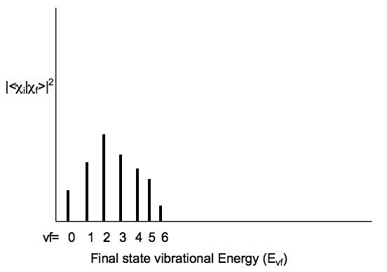
Notice that as one moves to higher vf values, the energy spacing between the states \((\text{E}_{vf} - \text{E}_{vf-1})\) decreases; this, of course, reflects the anharmonicity in the excited state vibrational potential. For the above example, the transition to the vf = 2 state has the largest FranckCondon factor. This means that the overlap of the initial state's vibrational wavefunction \(\chi_{vi} \text{ is largest for the final state's } \chi_{vf}\) function with vf = 2.
As a qualitative rule of thumb, the larger the geometry difference between the initial and final state potentials, the broader will be the Franck-Condon profile (as shown above) and the larger the vf value for which this profile peaks. Differences in harmonic frequencies between the two states can also broaden the Franck-Condon profile, although not as significantly as do geometry differences.
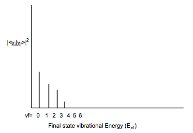
For example, if the initial and final states have very similar geometries and frequencies along the mode that is excited when the particular electronic excitation is realized, the following type of Franck-Condon profile may result:
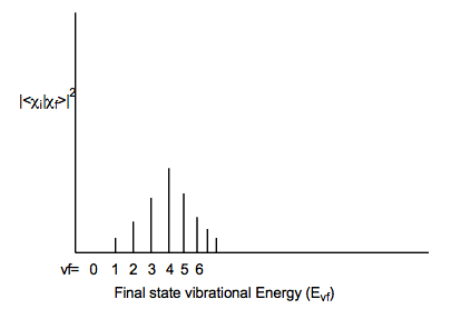
In contrast, if the initial and final electronic states have very different geometries and/or vibrational frequencies along some mode, a very broad Franck-Condon envelope peaked at high-vf will result as shown below:
Vibronic Effects
The second term in the above expansion of the transition dipole matrix element \( \sum\limits_a \dfrac{\partial \mu_{f,i}}{\partial R_a}(R_a - R_{a,e}) \) can become important to analyze when the first term \( \mu_{f,i}(\textbf{R}_e) \) vanishes (e.g., for reasons of symmetry). This dipole derivative term, when substituted into the integral over vibrational coordinates gives \( \sum\limits_a \dfrac{\partial \mu_{f,i}}{\partial R_a} \langle \chi_{vf} | (R_a - R_{a,e}) | \chi_{vi} \rangle \). Transitions for which \(\mu_{f,i}(\textbf{R}_e)\) vanishes but for which \( \dfrac{\partial \mu_{f,i}}{\partial R_a} \) does not for the \(\text{a}^{th}\) vibrational mode are said to derive intensity through "vibronic coupling" with that mode. The intensities of such modes are dependent on how strongly the electronic dipole integral varies along the mode (i.e, on \(\dfrac{\partial \mu_{f,i}}{\partial \textbf{R}_a}\) ) as well as on the magnitude of the vibrational integral \( \langle \chi_{vf} | ( R_a - R_{a,e}) | \chi_{vi} \rangle .\)
An example of an E1 forbidden but "vibronically allowed" transition is provided by the singlet n \(\rightarrow \pi^{\text{*}}\) transition of \(H_2CO\) that was discussed earlier in this section. As detailed there, the ground electronic state has \(^1\text{A}_1\) symmetry, and the n \(\rightarrow \pi^{\text{*}} \text{ state is of } ^1\text{A}_2\) symmetry, so the E1 transition integral \( \langle \psi_{ef} | \mu | \psi_{ei} \rangle \) vanishes for all three (x, y, z) components of the electric dipole operator \(\mu\). However, vibrations that are of \(\text{b}_2\) symmetry (e.g., the H-C-H asymmetric stretch vibration) can induce intensity in the n \(\rightarrow \pi^{\text{*}}\) transition as follows: (i) For such vibrations, the \(\text{b}_2\) mode's vi = 0 to vf = 1 vibronic integral \( \langle \chi_{vf} | (R_a - R_{a,e}) | \chi_{vi} \rangle \) will be non-zero and probably quite substantial (because, for harmonic oscillator functions these "fundamental" transition integrals are dominant- see earlier); (ii) Along these same \(\text{b}_2\) modes, the electronic transition dipole integral derivative \( \frac{\partial \mu_{f,i}}{\partial R_a} \) will be non-zero, even though the integral itself \(\mu_{f,i} (\textbf{R}_e)\) vanishes when evaluated at the initial state's equilibrium geometry.
To understand why the derivative \( \frac{\partial \mu_{f,i}}{\partial R_a}\) can be non-zero for distortions (denoted \(R_a) \text{ of b}_2\) symmetry, consider this quantity in greater detail:
\[ \dfrac{\partial \mu_{f,i}}{\partial R_a} = \dfrac{\partial}{\partial R} \langle \psi_{ef} | \mu | \psi_{ei} \rangle = \langle \dfrac{\partial \psi_{ef}}{\partial R_a} | \mu | \psi_{ei} \rangle + \langle \psi_{ef} | \mu | \dfrac{\partial \psi_{ei}}{\partial R_a} \rangle + \langle \psi_{ef} | \dfrac{\partial \mu}{\partial R_a} | \psi_{ei} \rangle . \nonumber \]
The third integral vanishes because the derivative of the dipole operator itself \( \mu = \sum\limits_i e r_j + \sum\limits_a Z_a e \text{R}_a\) with respect to the coordinates of atomic centers, yields an operator that contains only a sum of scalar quantities (the elementary charge e and the magnitudes of various atomic charges \(\text{Z}_a\)); as a result and because the integral over the electronic wavefunctions \( \langle \psi+{ef} | \psi_{ei} \rangle \) vanishes, this contribution yields zero. The first and second integrals need not vanish by symmetry because the wavefunction derivatives \( \frac{\partial \psi_{ef}}{\partial R_a} \text{ and} \frac{\partial \psi_{ei}}{\partial R_a} \) do not possess the same symmetry as their respective wavefunctions \(\psi_{ef} \text{ and } \psi_{ei}.\) In fact, it can be shown that the symmetry of such a derivative is given by the direct product of the symmetries of its wavefunction and the symmetry of the vibrational mode that gives rise to the \(\frac{\partial }{\partial R_a}. \text{ For the }H_2CO\) case at hand, the \(\text{b}_2\) mode vibration can induce in the excited \(^1\text{A}_2\) state a derivative component (i.e., \( \frac{\partial \psi_{ef}}{\partial R_a} \) ) that is of \(^1\text{B}_1\) symmetry) and this same vibration can induce in the \(^1\text{A}_1\) ground state a derivative component of \(^1\text{B}_2\) symmetry.
As a result, the contribution \( \langle \frac{\psi_{ef}}{\partial R_a} | \mu | \psi_{ei} \rangle \) to \( \frac{\partial \mu_{f,i}}{\partial R_a} \) arising from vibronic coupling within the excited electronic state can be expected to be non-zero for components of the dipole operator \(\mu\) that are of \( ( \frac{\partial \psi_{ef}}{\partial R_a} x \psi_{ei}) = (\text{B}_1 \text{ x A}_1) = \text{ B}_1 \) symmetry. Light polarized along the molecule's x-axis gives such a \(\text{b}_1\) component to \(\mu\) (see the \(\text{C}_{2v}\) character table in Appendix E). The second contribution \( \langle \psi_{ef} | \mu | \frac{\partial \psi_{ei}}{\partial R_a} \rangle \) can be non-zero for components of \(\mu\) that are of \( ( \psi+{ef} \text{ x }\frac{\partial \psi_{ei}}{\partial R_a}) \) = \( ( \text{A}_2 \text{ x B}_2 ) = \text{B}_1 \) symmetry; again, light of x-axis polarization can induce such a transition.
In summary, electronic transitions that are E1 forbidden by symmetry can derive significant (e.g., in \(H_2CO\) the singlet n \(\rightarrow \pi^{\text{*}}\) transition is rather intense) intensity through vibronic coupling. In such coupling, one or more vibrations (either in the initial or the final state) cause the respective electronic wavefunction to acquire (through \( \frac{\partial \psi}{\partial R_a} \)) a symmetry component that is different than that of \(\psi\) itself. The symmetry of \( \frac{\partial \psi}{\partial R_a} \), which is given as the direct product of the symmetry of \(\psi\) and that of the vibration, can then cause the electric dipole integral \( \langle \psi ' | \mu | \frac{\partial \psi}{\partial R_a} \rangle\) to be non-zero even when \( \langle \psi ' | \mu | \psi \rangle \)is zero. Such vibronically allowed transitions are said to derive their intensity through vibronic borrowing.
Rotational Selection Rules for Electronic Transitions
Each vibrational peak within an electronic transition can also display rotational structure (depending on the spacing of the rotational lines, the resolution of the spectrometer, and the presence or absence of substantial line broadening effects such as those discussed later in this Chapter). The selection rules for such transitions are derived in a fashion that parallels that given above for the vibration-rotation case. The major difference between this electronic case and the earlier situation is that the vibrational transition dipole moment \(\mu_{\text{trans}}\) appropriate to the former is replaced by \(\mu_{f,i}(\textbf{R}_e)\) for conventional (i.e., nonvibronic) transitions or \( \frac{\partial \mu_{f,i}}{\partial R_a} \) (for vibronic transitions).
As before, when \(\mu_{f,i}(\textbf{R}_e) \text{( or } \frac{\partial \mu_{f,i}}{\partial \textbf{R}_a})\) lies along the molecular axis of a linear molecule, the transition is denoted \(\sigma\) and k = 0 applies; when this vector lies perpendicular to the axis it is called \(\pi\) and k = ±1 pertains. The resultant linear-molecule rotational selection rules are the same as in the vibration-rotation case:
\[ \Delta L = \pm 1, \text{ and } \Delta M = \pm 1,0 \text{ (for } \sigma \text{ transitions).} \nonumber \]
\[ \Delta L = \pm 1, \text{ and } \Delta M = \pm 1,0 \text{ (for } \pi \text{ transitions).} \nonumber \]
In the latter case, the L = L' = 0 situation does not arise because a p transition has one unit of angular momentum along the molecular axis which would preclude both L and L' vanishing.
\[ \Delta L = \pm 1,0; \Delta M = \pm 1,0; \text{ and } \Delta K = 0 \text{ (L = L' = 0 is not allowed and all } \Delta L = 0 \text{ are forbidden when K = K' = 0) } \nonumber \]
which applies when \( \mu_{f,i}(\textbf{R}_e) \text{ or } \frac{\partial \mu_{f,i}}{\partial R_a}\) lies along the symmertry axis, and
\[ \Delta L = \pm 1,0; \Delta M = \pm 1,0; \text{ and } \Delta K = \pm 1 \text{ (L = L' = 0 is not allowed)} \nonumber \]
which applies when \(\mu_{f,i}(\textbf{R}_e) \text{ or } \frac{\partial \mu_{f,i}}{\partial R_a}\) lies perpendicular to the symmetry axis.