14.3: Application to Electromagnetic Perturbations

First-Order Fermi-Wentzel "Golden Rule"

Using the earlier expressions for \(H^1_{int}\) and for A(r,t)

\[ H^1_{int} = \sum\limits_j \left[ \left( \dfrac{ie\hbar}{m_ec} \right) \textbf{A}(r_j,t) \cdot{\nabla_j} \right] + \sum\limits_a \left[ \left( \dfrac{iZ_ae\hbar}{m_ac} \right) \textbf{A}(R_a,t) \cdot{\nabla_a} \right] \nonumber \]

and

\[ 2\textbf{A}_o cos(\omega t - \textbf{k}\cdot{\textbf{r}}) = \textbf{A}_0 \left[ e^{i(\omega t - \textbf{k}\cdot{\textbf{r}})} + e^{-i(\omega t - \textbf{k}\cdot{\textbf{r}})} \right], \nonumber \]

it is relatively straightforward to carry out the above time integration to achieve a final expression for \(D_f^1(t)\), which can then be substituted into \(C_f^1(t) = D_f^1(t) e^{(-\frac{-iE_f^0t}{\hbar})}\) to obtain the final expression for the first-order estimate of the probability amplitude for the molecule appearing in the state \(\Phi_f e^{\frac{-iE_f^0t}{\hbar}}\) after being subjected to electromagnetic radiation from t = 0 until t = T. This final expression reads:

\[ C_f^1(T) = \dfrac{1}{i\hbar} e^{\dfrac{-iE_f^0T}{\hbar}} \left[ \langle\Phi_f|\sum\limits_j \left[ \left( \dfrac{ie\hbar}{m_ec} \right) e^{-i\textbf{k}\cdot{\textbf{r}_j}}\textbf{A}_0\cdot{\nabla_j} + \sum\limits_a \left( \dfrac{iZ_ae\hbar}{m_ac} \right) e^{-i\textbf{k}\cdot{R}_a}\textbf{A}_0\cdot{\nabla_a}|\Phi_i \rangle \right] \dfrac{e^{i(\omega + \omega_{f,i})T}-1}{i(\omega + \omega_{f,i})} \right] \nonumber \]

\[ + \dfrac{1}{i\hbar} e^{\dfrac{-iE_f^0T}{\hbar}}\left[\langle\Phi_f|\sum\limits_j \left[ \left( \dfrac{ie\hbar}{m_ec} \right) e^{i\textbf{k}\cdot{\textbf{r}_j}}\textbf{A}_0\cdot{\nabla_j} + \sum\limits_a \left( \dfrac{iZ_ae\hbar}{m_ac} \right) e^{i\textbf{k}\cdot{R}_a}\textbf{A}_0\cdot{\nabla_a}|\Phi_i \rangle \right] \dfrac{e^{i(-\omega + \omega_{f,i})T}-1}{i(-\omega + \omega_{f,i})} \right] \nonumber \]

where

\[ \omega_{f,i} = \dfrac{[E_f^0 - E_i^0]}{\hbar} \nonumber \]

is the resonance frequency for the transition between "initial" state \(\Phi_i \text{ and "final" state } \Phi_f\)

Defining the time-independent parts of the above expression as

\[ \alpha_{f,i} = \langle \Phi_f |\sum\limits_j \left[ \left( \dfrac{e}{m_ec} \right) e^{-i\textbf{k}\cdot{\textbf{r}_j}}\textbf{A}_0\cdot{\nabla_j} + \sum\limits_a \left( \dfrac{Z_ae}{m_ac} \right) e^{-i\textbf{k}\cdot{\textbf{R}_a}}\textbf{A}_0\cdot{\nabla_a}|\Phi_i \rangle, \right] \nonumber \]

this result can be written as

\[ C_f^1(T) = e^{\dfrac{-iE_f^0T}{\hbar}}\left[ \alpha_{f,i}\dfrac{e^{i(\omega+\omega_{f,i})T}-1}{i(\omega+\omega_{f,i})} + \alpha^{\text{*}}_{f,i}\dfrac{e^{-i(\omega - \omega_{f,i})T}-1}{-i(\omega-\omega_{f,i})} \right]. \nonumber \]

The modulus squared \(|C_f^1(T)|^2\) gives the probability of finding the molecule in the final state \(\Phi_f\) at time T, given that it was in \(\Phi_i\) at time t = 0. If the light's frequency \(\omega\) is tuned close to the transition frequency \(\omega_{f,i}\) of a particular transition, the term whose denominator contains \((\omega - \omega_{f,i})\) will dominate the term with \((\omega + \omega_{f,i})\) in its denominator. Within this "near-resonance" condition, the above probability reduces to:

\[ |C_f^1|^2 = 2|\alpha_{f,i}|^2 \dfrac{1-cos(\omega - \omega_{f,i})T}{(\omega - \omega_{f,i})^2} \nonumber \]

\[ = 4|\alpha_{f,i}|^2\dfrac{sin^2(1/2(\omega - \omega_{f,i})T)}{(\omega - \omega_{f,i})^2}. \nonumber \]

This is the final result of the first-order time-dependent perturbation theory treatment of light-induced transitions between states \(\Phi_i \text{ and } \Phi_f\).

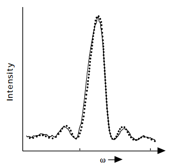
The so-called sinc-function

\[ \dfrac{sin^2(1/2(\omega - \omega_{f,i})T)}{(\omega - \omega_{f,i})^2} \nonumber \]

as shown in the figure below is strongly peaked near \(\omega = \omega_{f,i}\), and displays secondary maxima (of decreasing amplitudes) near \(\omega = \omega_{f,i} + 2\frac{n\pi}{T} , n = 1, 2\), ... . In the \(T \rightarrow \infty\) limit, this function becomes narrower and narrower, and the area under it

\[ \int\limits_{-\infty}^{\infty} \dfrac{sin^2(1/2(\omega - \omega_{f,i})T)}{(\omega - \omega_{f,i})^2}d\omega = \dfrac{T}{2}\int\limits_{-\infty}^{\infty} \dfrac{sin^2(1/2(\omega - \omega_{f,i})T)}{1/4T^2(\omega - \omega_{f,i})^2}d\left(\omega \dfrac{T}{2}\right) = \dfrac{T}{2}\int\limits_{-\infty}^{\infty} \dfrac{sin^2(x)}{x^2} = \pi\dfrac{T}{2} \nonumber \]

grows with T. Physically, this means that when the molecules are exposed to the light source for long times (large T), the sinc function emphasizes \(\omega\) values near \(\omega_{f,i}\) (i.e., the on-resonance \(\omega\) values). These properties of the sinc function will play important roles in what follows.

Figure 14.3.1: Insert caption here!

In most experiments, light sources have a "spread" of frequencies associated with them; that is, they provide photons of various frequencies. To characterize such sources, it is common to introduce the spectral source function g(\(\omega\)) d\(\omega\) which gives the probability that the photons from this source have frequency somewhere between \(\omega \text{ and } \omega+d\omega\). For narrow-band lasers, g(\(\omega)\) is a sharply peaked function about some "nominal" frequency \(\omega_o\); broader band light sources have much broader g(\(\omega\)) functions.

When such non-monochromatic light sources are used, it is necessary to average the above formula for \(|C_f^1(T)|^2\) over the g(\(\omega\)) d\(\omega\) probability function in computing the probability of finding the molecule in state \(\Phi_f\) after time T, given that it was in \(\Phi_i\) up until t = 0, when the light source was turned on. In particular, the proper expression becomes:

\[ |C_f^1(T)|^2_{ave} = 4|\alpha_{fi}|^2 \int\limits g(\omega) \dfrac{sin^2(1/2(\omega - \omega_{f,i})T)}{(\omega - \omega_{f,i})^2}d\omega \nonumber \]

\[ = 2|\alpha_{f,i}|^2 T \int\limits_{-\infty}^{\infty} g(\omega) \dfrac{2in^2(1/2(\omega - \omega_{f,i})T)}{1/4T^2(\omega - \omega_{f,i})^2}d\left( \omega\dfrac{T}{2}\right) \nonumber \]

If the light-source function is "tuned" to peak near \(\omega = \omega_{f,i}\) and if \(g(\omega)\) is much broader (in \(\omega\)-space) than the \( \dfrac{sin^2(1/2(\omega - \omega_{f,i})T)}{(\omega - \omega_{f,i})^2} \) function, g(\(\omega\)) can be replaced by its value at the peak of the \( \dfrac{sin^2(1/2(\omega - \omega_{f,i})T)}{(\omega - \omega_{f,i})^2} \) function, yielding:

\[ |C_f^1(T)_{ave} = 2g(\omega_{f,i})|\alpha_{f,i}|^2T \int\limits^{\infty}_{-\infty}\dfrac{sin^2(1/2(\omega - \omega_{f,i})T}{1/4T^2(\omega - \omega_{f,i})^2}d\left( \omega\dfrac{T}{2} \right) = 2g(\omega_{f,i})|\alpha_{f,i}|^2 T\int\limits_{-\infty}^{\infty} \dfrac{sin^2(x)}{x^2}dx = 2\pi g(\omega_{f,i})|\alpha_{f,i}|^2T. \nonumber \]

The fact that the probability of excitation from \(\Phi_i \text{ to } \Phi_f\) grows linearly with the time T over which the light source is turned on implies that the rate of transitions between these two states is constant and given by:

\[ \textbf{R}_{i,f} = 2\pi g(\omega_{f,i})|\alpha_{f,i}|^2; \nonumber \]

this is the so-called first-order Fermi-Wentzel "golden rule" expression for such transition rates. It gives the rate as the square of a transition matrix element between the two states involved, of the first order perturbation multiplied by the light source function \(g(\omega)\) evaluated at the transition frequency \(\omega_{f,i}\).

Higher Order Results

Solution of the second-order time-dependent perturbation equations,

\[ i\hbar\dfrac{\partial \Psi^2}{\partial t} = (H^0\Psi^2 + H^2_{int}\Psi^0 + H^1_{int}\Psi^1) \nonumber \]

which will not be treated in detail here, gives rise to two distinct types of contributions to the transition probabilities between \(\Phi_i \text{ and } \Phi_f\):

There will be matrix elements of the form

\[ \langle \Phi_f | \sum\limits_j \left[ \left( \dfrac{e^2}{2m_ec^2} \right)| \textbf{A}(\textbf{r}_j,t)|^2 \right] + \sum\limits_a\left[ \left( \dfrac{Z_a^2e^2}{2m_ac^2} \right)|\textbf{A}(R_a,t)|^2 \right]|\Phi_i \rangle \nonumber \]

arising when \(H^2_{int} \text{ couples } \Phi_i \text{ to } \Phi_f\).

There will be matrix elements of the form

\[ \sum\limits_k <\Phi_f |\sum\limits_j \left[ \left( \dfrac{ie\hbar}{m_ec} \right)\textbf{A}(r_j,t)\cdot{\nabla_j} \right] + \sum\limits_a \left[ \left( \dfrac{iZ_ae\hbar}{m_ac} \right)\textbf{A}(R_a,t)\cdot{\nabla_a} \right]| \Phi_k \rangle \nonumber \]

\[ \langle\Phi_k |\sum\limits_j \left[ \left( \dfrac{ie\hbar}{m_ec} \right)\textbf{A}(r_j,t)\cdot{\nabla_j} \right] + \sum\limits_a \left[ \left( \dfrac{iZ_ae\hbar}{m_ac} \right)\textbf{A}(R_a,t)\cdot{\nabla_a} \right]| \Phi_i \rangle \nonumber \]

arising from expanding \( H^1_{int}\Psi^1 = \sum\limits_kC_k^1H^1_{int}|\Phi_k \rangle \) and using the earlier result for the first-order amplitudes \(C_k^1\). Because both types of second-order terms vary quadratically with the A(r,t) potential, and because A has time dependence of the form \(cos(\omega t - \textbf{k}\cdot{\textbf{r}})\), these terms contain portions that vary with time as \(cos(2\omega t).\) As a result, transitions between initial and final states \(\Phi_i \text{ and } \Phi_f\) whose transition frequency is \(\omega_{f,i}\) can be induced when \(2\omega = \omega_{f,i}\); in this case, one speaks of coherent two-photon induced transitions in which the electromagnetic field produces a perturbation that has twice the frequency of the "nominal" light source frequency \(\omega\).