5.3: Linear Molecules

Linear molecules belong to the axial rotation group. Their symmetry is intermediate in complexity between nonlinear molecules and atoms.

For linear molecules, the symmetry of the electrostatic potential provided by the nuclei and the other electrons is described by either the \(C_{\infty n} \text{ or } D_{\infty h}\) group. The essential difference between these symmetry groups and the finite point groups which characterize the non-linear molecules lies in the fact that the electrostatic potential which an electron feels is invariant to rotations of any amount about the molecular axis (i.e., V(\(\gamma +\delta \gamma ) =V(\gamma\)), for any angle increment \(\delta\gamma\)). This means that the operator \(C_{\delta\gamma}\) which generates a rotation of the electron's azimuthal angle \(\gamma\) by an amount \(\delta\gamma\) about the molecular axis commutes with the Hamiltonian [h, \(C_{\delta\gamma}\) ] =0. \(C_{\delta\gamma}\) can be written in terms of the quantum mechanical operator \(L_z = -i\hbar \frac{\partial}{\partial \gamma}\) describing the orbital angular momentum of the electron about the molecular (z) axis:

\[ C_{\delta\gamma}= e^{i\delta\gamma\dfrac{L_z}{\hbar}}. \nonumber \]

Because \(C_{\delta\gamma}\) commutes with the Hamiltonian and \(C_{\delta\gamma}\) can be written in terms of \(L_z , L_z\) must commute with the Hamiltonian. As a result, the molecular orbitals \(\phi\) of a linear molecule must be eigenfunctions of the z-component of angular momentum \(L_z\):

\[ -i\hbar\dfrac{\partial}{\partial y}| \phi \rangle = m\hbar | \phi \rangle. \nonumber \]

The electrostatic potential is not invariant under rotations of the electron about the x or y axes (those perpendicular to the molecular axis), so \(L_x \text{ and } L_y\) do not commute with the Hamiltonian. Therefore, only \(L_z\) provides a "good quantum number" in the sense that the operator \(L_z\) commutes with the Hamiltonian.

In summary, the molecular orbitals of a linear molecule can be labeled by their m quantum number, which plays the same role as the point group labels did for non-linear polyatomic molecules, and which gives the eigenvalue of the angular momentum of the orbital about the molecule's symmetry axis. Because the kinetic energy part of the Hamiltonian contains \( \frac{\hbar^2}{2m_er^2}\frac{\partial^2}{\partial \gamma^2} \), whereas the potential energy part is independent of \(\gamma\), the energies of the molecular orbitals depend on the square of the m quantum number. Thus, pairs of orbitals with m= ± 1 are energetically degenerate; pairs with m= ± 2 are degenerate, and so on. The absolute value of m, which is what the energy depends on, is called the \(\lambda\) quantum number. Molecular orbitals with \(\lambda = 0 \text{ are called } \sigma\) orbitals; those with \(\lambda = 1 \text{ are } \pi\) orbitals; and those with \(\lambda\) = 2 are \(\delta\) orbitals.

Just as in the non-linear polyatomic-molecule case, the atomic orbitals which constitute a given molecular orbital must have the same symmetry as that of the molecular orbital. This means that \(\sigma,\pi, \text{ and } \delta\) molecular orbitals are formed, via LCAO-MO, from m=0, m= ± 1, and m= ± 2 atomic orbitals, respectively. In the diatomic \(N_2\) molecule, for example, the core orbitals are of \(\sigma\) symmetry as are the molecular orbitals formed from the 2s and \(2p_z\) atomic orbitals (or their hybrids) on each Nitrogen atom. The molecular orbitals formed from the atomic \(2p_{-1} =(2p_x- i2p_y) \text{ and the } 2p_{+1} = (2p_x + i2p_y\)) orbitals are of p symmetry and have m = -1 and +1.

For homonuclear diatomic molecules and other linear molecules which have a center of symmetry, the inversion operation (in which an electron's coordinates are inverted through the center of symmetry of the molecule) is also a symmetry operation. Each resultant molecular orbital can then also be labeled by a quantum number denoting its parity with respect to inversion. The symbols g (for gerade or even) and u (for ungerade or odd) are used for this label. Again for \(N_2\), the core orbitals are of \(\sigma_g \text{ and } \sigma_u\) symmetry, and the bonding and antibonding \(\sigma\) orbitals formed from the 2s and \(2p_\sigma\) orbitals on the two Nitrogen atoms are of \(\sigma_g \text{ and } \sigma_u\) symmetry.

Figure 5.4.1: Insert caption here!

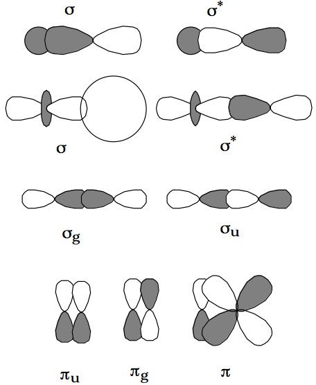
The bonding \(\pi\) molecular orbital pair (with m = +1 and -1) is of \(\pi_u\) symmetry whereas the corresponding antibonding orbital is of \(\pi_g\) symmetry. Examples of such molecular orbital symmetries are shown above.

The use of hybrid orbitals can be illustrated in the linear-molecule case by considering the \(N_2\) molecule. Because two \(\pi\) bonding and antibonding molecular orbital pairs are involved in \(N_2\) (one with m = +1, one with m = -1), VSEPR theory guides one to form sp hybrid orbitals from each of the Nitrogen atom's 2s and \(2p_z\) (which is also the 2p orbital with m = 0) orbitals. Ignoring the core orbitals, which are of \(\sigma_g \text{ and } \sigma_u\) symmetry as noted above, one then symmetry adapts the four sp hybrids (two from each atom) to build one \(\sigma_g\) orbital involving a bonding interaction between two sp hybrids pointed toward one another, an antibonding \(\sigma_u\) orbital involving the same pair of sp orbitals but coupled with opposite signs, a nonbonding \(\sigma_g\) orbital composed of two sp hybrids pointed away from the interatomic region combined with like sign, and a nonbonding \(\sigma_u\) orbital made of the latter two sp hybrids combined with opposite signs. The two \(2p_m\) orbitals (m= +1 and -1) on each Nitrogen atom are then symmetry adapted to produce a pair of bonding \(\pi_u\) orbitals (with m = +1 and -1) and a pair of antibonding \(\pi_g\) orbitals (with m = +1 and -1). This hybridization and symmetry adaptation thereby reduces the 8x8 secular problem (which would be 10x10 if the core orbitals were included) into a 2x2 \(\sigma_g\) problem (one bonding and one nonbonding), a 2x2 \(\sigma_u\) problem (one bonding and one nonbonding), an identical pair of 1x1 \(\pi_u\) problems (bonding), and an identical pair of 1x1 \(\pi_g\) problems (antibonding).

Another example of the equivalence among various hybrid and atomic orbital points of view is provided by the CO molecule. Using, for example, sp hybrid orbitals on C and O, one obtains a picture in which there are: two core \(\sigma\) orbitals corresponding to the O-atom 1s and C-atom 1s orbitals; one CO bonding, two non-bonding, and one CO antibonding orbitals arising from the four sp hybrids; a pair of bonding and a pair of antibonding \(\pi\) orbitals formed from the two p orbitals on O and the two p orbitals on C. Alternatively, using \(sp^2\) hybrids on both C and O, one obtains: the two core \(\sigma\) orbitals as above; a CO bonding and antibonding orbital pair formed from the \(sp^2\) hybrids that are directed along the CO bond; and a single \(\pi\) bonding and antibonding \(\pi^{\text{*}}\) orbital set. The remaining two \(sp^2\) orbitals on C and the two on O can then be symmetry adapted by forming ± combinations within each pair to yield: an \(a_1\) non-bonding orbital (from the + combination) on each of C and O directed away from the CO bond axis; and a \(p_\pi\) orbital on each of C and O that can subsequently overlap to form the second \(\pi\) bonding and \(\pi^{\text{*}}\) antibonding orbital pair.

It should be clear from the above examples, that no matter what particular hybrid orbitals one chooses to utilize in conceptualizing a molecule's orbital interactions, symmetry ultimately returns to force one to form proper symmetry adapted combinations which, in turn, renders the various points of view equivalent. In the above examples and in several earlier examples, symmetry adaptation of, for example, \(sp^2\) orbital pairs (e.g., \(sp_L^2 ± sp_R^2\)) generated orbitals of pure spatial symmetry. In fact, symmetry combining hybrid orbitals in this manner amounts to forming other hybrid orbitals. For example, the above ± combinations of \(sp^2\) hybrids directed to the left (L) and right (R) of some bond axis generate a new sp hybrid directed along the bond axis but opposite to the \(sp^2\) hybrid used to form the bond and a non-hybridized p orbital directed along the L-to-R direction. In the CO example, these combinations of \(sp^2\) hybrids on O and C produce sp hybrids on O and C and \(p_\pi\) orbitals on O and C.