5.3: Fourier Transform Spectroscopy

Last updated
Save as PDF

Page ID: 298973

\( \newcommand{\vecs}[1]{\overset { \scriptstyle \rightharpoonup} {\mathbf{#1}} } \) \( \newcommand{\vecd}[1]{\overset{-\!-\!\rightharpoonup}{\vphantom{a}\smash {#1}}} \)\(\newcommand{\id}{\mathrm{id}}\) \( \newcommand{\Span}{\mathrm{span}}\) \( \newcommand{\kernel}{\mathrm{null}\,}\) \( \newcommand{\range}{\mathrm{range}\,}\) \( \newcommand{\RealPart}{\mathrm{Re}}\) \( \newcommand{\ImaginaryPart}{\mathrm{Im}}\) \( \newcommand{\Argument}{\mathrm{Arg}}\) \( \newcommand{\norm}[1]{\| #1 \|}\) \( \newcommand{\inner}[2]{\langle #1, #2 \rangle}\) \( \newcommand{\Span}{\mathrm{span}}\) \(\newcommand{\id}{\mathrm{id}}\) \( \newcommand{\Span}{\mathrm{span}}\) \( \newcommand{\kernel}{\mathrm{null}\,}\) \( \newcommand{\range}{\mathrm{range}\,}\) \( \newcommand{\RealPart}{\mathrm{Re}}\) \( \newcommand{\ImaginaryPart}{\mathrm{Im}}\) \( \newcommand{\Argument}{\mathrm{Arg}}\) \( \newcommand{\norm}[1]{\| #1 \|}\) \( \newcommand{\inner}[2]{\langle #1, #2 \rangle}\) \( \newcommand{\Span}{\mathrm{span}}\)\(\newcommand{\AA}{\unicode[.8,0]{x212B}}\)

The last example underscores the close relationship between time and frequency domain representations of the data. Similar information to the frequency-domain double resonance experiment is obtained by Fourier transformation of the coherent evolution periods in a time domain experiment with short broadband pulses.

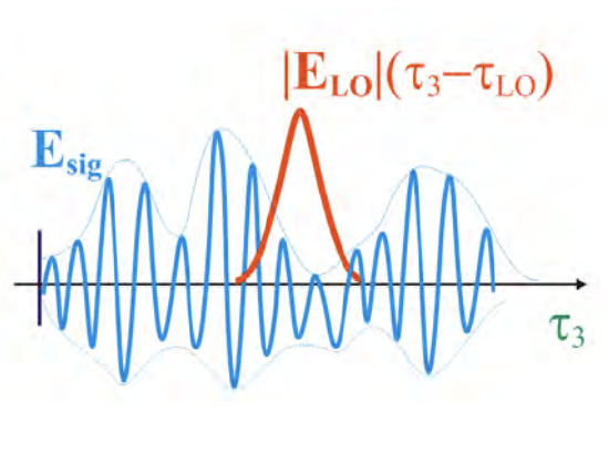
In practice, the use of Fourier transforms requires a phase-sensitive measure of the radiated signal field, rather than the intensity measured by photodetectors. This can be obtained by beating the signal against a reference pulse (or local oscillator) on a photodetector. If we measure the cross term between a weak signal and strong local oscillator:

\[\begin{aligned} \delta I_{LO}(\tau_{LO}) &= |E_{sig}+E_{LO}|^2-|E_{LO}|^2 \\ &\approx 2Re\int_{-\infty}^{+\infty}d\tau_3 E_{sig}(\tau_3)E_{LO}(\tau_3-\tau_{LO}) \end{aligned} \label{8.1}\]

For a short pulse \(E_{LO},\delta I(\tau_{LO})\propto E_{sig}(\tau_{LO})\). By acquiring the signal as a function of \(\tau_1\) and \(\tau_{LO}\) we can obtain the time domain signal and numerically Fourier transform to obtain a 2D spectrum.

Alternatively, we can perform these operations in reverse order, using a grating or other dispersive optic to spatially disperse the frequency components of the signal. This is in essence an analog Fourier Transform. The interference between the spatially dispersed Fourier components of the signal and LO are subsequently detected.

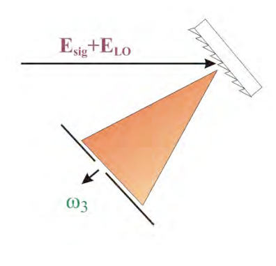
\[\delta I(\omega_3)=\int|E_{LO}(\omega_3)+E_{sig}(\omega_3)|^2-|E_{LO}(\omega_3)|^2 \nonumber\]