3.4: Pump-Probe

The pump-probe or transient absorption experiment is perhaps the most widely used third-order nonlinear experiment. It can be used to follow many types of time-dependent relaxation processes and chemical dynamics, and is most commonly used to follow population relaxation, chemical kinetics, or wavepacket dynamics and quantum beats.

The principle is quite simple, and the using the theoretical formalism of nonlinear spectroscopy often unnecessary to interpret the experiment. Two pulses separated by a delay \(\tau\) are crossed in a sample: a pump pulse and a time-delayed probe pulse. The pump pulse \(E_{pu}\) creates a non-equilibrium state, and the time-dependent changes in the sample are characterized by the probe-pulse \(E_{pr}\) through the pump-induced intensity change on the transmitted probe, \(\Delta I\).

Described as a third-order coherent nonlinear spectroscopy, the signal is radiated collinear to the transmitted probe field, so the wavevector matching condition is

\[\bar k_{sig}=+\bar k_{pu} -\bar k_{pu} +\bar k_{pr}=\bar k_{pr}.\]

There are two interactions with the pump field and the third interaction is with the probe. Similar to the transient grating, the time-ordering of pump-interactions cannot be distinguished, so terms that contribute to scattering along the probe are \(k_{sig}=\pm k_1 \mp k_2 + k_3\) (i.e., all correlation functions R₁ to R₄). In fact, the pump-probe can be thought of as the limit of the transient grating experiment in the limit of zero grating wavevector (\(\theta\) and \(\beta\rightarrow 0\)).

The detector observes the intensity of the transmitted probe and nonlinear signal

\[I=\frac{nc}{4\pi}|E_{pr}'+E_{sig}|^2 \label{4.4.1}\]

\(E_{pr}'\) is the transmitted probe field corrected for linear propagation through the sample. The measured signal is typically the differential intensity on the probe field with and without the pump field present:

\[\Delta I(\tau)=\frac{nc}{4\pi}\left\{|E_{pr}'+E_{sig}(\tau)|^2-|E_{pr}'|^2\right\} \label{4.4.2}\]

If we work under conditions of a weak signal relative to the transmitted probe \(|E_{pr}'|\gt\gt|E_{sig}|\), then the differential intensity in eq. (4.4.2) is dominated by the cross term

\[\begin{aligned} \Delta I(\tau) & \approx \frac{n c}{4 \pi}\left[E_{p r}^{\prime} E_{s i g}^{*}(\tau)+c . c .\right] \\ &=\frac{n c}{2 \pi} \operatorname{Re}\left[E_{p r}^{\prime} E_{s i g}^{*}(\tau)\right] \end{aligned}\label{4.4.3}\]

So the pump-probe signal is directly proportional to the nonlinear response. Since the signal field is related to the nonlinear polarization through a \(\pi/2) phase shift,

\[\bar E_{sig}(\tau)=i\frac{2\pi\omega_{sig}\ell}{nc}P^{(3)}(\tau)\label{4.4.4}\]

the measured pump-probe signal is proportional to the imaginary part of the polarization

\[\Delta I(\tau)=2\omega_{sig}\ell Im\left[E_{pr}'P^{(3)}(\tau)\right]\label{4.4.5}\]

which is also proportional to the correlation functions derived from the resonant diagrams we considered earlier.

Dichroic and Birefringent Response

In analogy to what we observed earlier for linear spectroscopy, the nonlinear changes in absorption of the transmitted probe field are related to the imaginary part of the susceptibility, or the imaginary part of the index of refraction. In addition to the fully resonant processes, it is also possible for the pump field to induce nonresonant changes to the polarization that modulate the real part of the index of refraction. These can be described through a variety of nonresonant interactions, such as nonresonant Raman, the optical Kerr effect, coherent Raleigh or Brillouin scattering, or the second hyperpolarizability of the sample. In this case, we can describe the timedevelopment of the polarization and radiated signal field as

\[\begin{aligned} P^{(3)}(\tau,\tau_3) &= P^{(3)}(\tau,\tau_3)e^{-i\omega_{sig}\tau_3}+\left[P^{(3)}(\tau,\tau_3)\right]^*e^{i\omega_{sig}}\tau_3 \\ &= 2Re\left[P^{(3)}(\tau,\tau_3)\right]\cos{(\omega_{sig}\tau_3)}+2Im\left[P^{(3)}(\tau,\tau_3)\right]\sin{(\omega_{sig}\tau_3)} \end{aligned}\label{4.4.6}\]

\[\begin{aligned}\bar E_{sig}(\tau_3) &=\frac{4\pi\omega_{sig}\ell}{nc}\left(Re\left[P^{(3)}(\tau,\tau_3)\right]\sin{(\omega_{sig}\tau_3)}+Im\left[P^{(3)}(\tau,\tau_3)\right]\cos{(\omega_{sig}\tau_3)}\right) \\ &= E_{bir}(\tau,\tau_3)\sin{(\omega_{sig}\tau_3)}+E_{dic}(\tau,\tau_3)\cos{(\omega_{sig}\tau_3)} \end{aligned}\label{4.4.7}\]

Here the signal is expressed as a sum of two contributions, referred to as the birefringent \((E_{bir})\) and dichroic \((E_{dic})\) responses. As before the imaginary part, or dichroic response, describes the sample-induced amplitude variation in the signal field, whereas the birefringent response corresponds to the real part of the nonlinear polarization and represents the phase-shift or retardance of the signal field induced by the sample.

In this scheme, the transmitted probe is

\[\bar E_{pr}'(\tau_3)=E_{pr}'(\tau_3)\cos{(\omega_{pr}\tau_3)} \label{4.4.8}\]

So that the

\[\Delta I(\tau)\approx\frac{nc}{2\pi}\left[E_{pr}'(\tau)E_{dic}(\tau)\right] \label{4.4.9}\]

Because the signal is in-quadrature with the polarization (\(\pi/2\) phase shift), the absorptive or dichroic response is in-phase with the transmitted probe, whereas the birefringent part is not observed. If we allow for the phase of the probe field to be controlled, for instance through a quarter-wave plate before the sample, then we can write

\[\bar E_{pr}'(\tau_3,\phi)=E_{pr}'(\tau_3)\cos{(\omega_{pr}\tau_3+\phi)} \label{4.4.10}\]

\[I(\tau,\phi)\approx\frac{nc}{2\pi}\left[E_{pr}'(\tau)E_{bir}(\tau)\sin{(\phi)}+E_{pr}'(\tau)E_{dic}(\tau)\cos{(\phi)}\right] \label{4.4.11}\]

The birefringent and dichroic response of the molecular system can now be observed for phases of \(\phi=\pi/2,3\pi/2\dots\) and \(\phi=0,\pi\dots\), respectively.

Incoherent pump-probe experiments

What information does the pump-probe experiment contain? Since the time delay we control is the second time interval \(\tau_2\), the diagrams for a two level system indicate that these measure population relaxation:

\[\Delta I(\tau)\propto|\mu_{ab}|^4e^{-\Gamma_{bb}\tau} \label{4.4.12}\]

In fact measuring population changes and relaxation are the most common use of this experiment. When dephasing is very rapid, the pump-probe can be interpreted as an incoherent experiment, and the differential intensity (or absorption) change is proportional to the change of population of the states observed by the probe field. The pump-induced population changes in the probe states can be described by rate equations that describe the population relaxation, redistribution, or chemical kinetics. For the case where the pump and probe frequencies are the same, the signal decays as a results of population relaxation of the initially excited state. The two-level system diagrams indicate that the evolution in \(\tau_2\) is differentiated by evolution in the ground or excited state. These diagrams reflect the equal signal contributions from the ground state bleach (loss of ground state population) and stimulated emission from the excited state. For direct relaxation from excited to ground state the loss of population in the excited state \(\Gamma_{bb}\) is the same as the refilling of the hole in the ground state \(\Gamma_{aa}\), so that \(\Gamma_{aa}=\Gamma_{bb}\). If population relaxation from the excited state is through an intermediate, then the pump-probe decay will reflect equal contributions from both processes, which can be described by coupled first-order rate equations.

When the resonance frequencies of the pump and probe fields are different, then the incoherent pump-probe signal is related to the joint probability of exciting the system at \(\omega_{pu}\) and detecting at \(\omega_{pr}\) after waiting a time \(\tau\), \(P(\omega_{pr},\tau;\omega_{pu})\).

Coherent pump-probe experiments

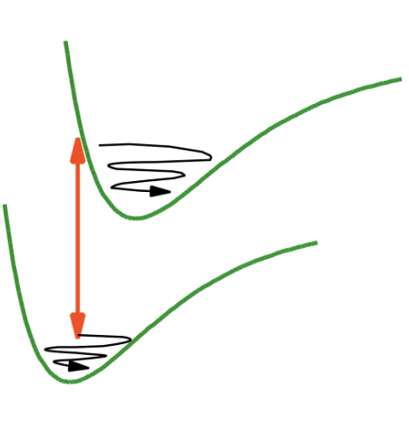
Ultrafast pump-probe measurements on the timescale of vibrational dephasing operate in a coherent regime where wavepackets prepared by the pump-pulse modulate the probe intensity. This provides a mechanism for studying the dynamics of excited electronic states with coupled vibrations and photoinitiated chemical reaction dynamics. If we consider the case of pump-probe experiments on electronic states where \(\omega_{pu}=\omega_{pr}\), our description of the pump-probe from Feynmann diagrams indicates that the pump-pulse creates excitations both on the excited state and ground state. Both wavepackets will contribute to the signal.

There are two equivalent ways of describing the experiment, which mirror our earlier description of electronic spectroscopy for an electronic transition coupled to nuclear motion. The first is to describe the spectroscopy in terms of the eigenstates of \(H_0, |e,n\rangle\). The second draws on the energy gap Hamiltonian to describe the spectroscopy as two electronic levels \(H_S\) that interact with the vibrational degrees of freedom \(H_B\), and the wavepacket dynamics are captured by \(H_{SB}\).

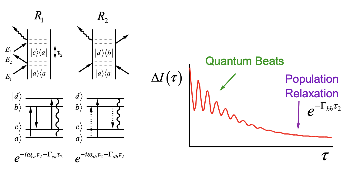
For the eigenstate description, a two level system is inadequate to capture the wavepacket dynamics. Instead, describe the spectroscopy in terms of the four-level system diagrams given earlier. In addition to the population relaxation terms, we see that the R₂ and R₄ terms describe the evolution of coherences in the excited electronic state, whereas the R₁ and R₃ terms describe the ground state wave packet. For an underdamped wavepacket these coherences are observed as quantum beats on the pump-probe signal.