3.3: Transient Grating

The transient grating is a third-order technique used for characterizing numerous relaxation processes, but is uniquely suited for looking at optical excitations with well-defined spatial period. The first two pulses are set time-coincident, so you cannot distinguish which field interacts first. Therefore, the signal will have contributions both from \(k_{sig} = k_1 − k_2 + k_3\) and \(k_{sig} = −k_1 + k_2 + k_3\). That is the signal depends on \(R_1+R_2+R_3+R_4\). Consider the terms contributing to the polarization that arise from the first two interactions. For two time-coincident pulses of the same frequency, the first two fields have an excitation profile in the sample

\[\bar E_a\bar E_b=E_aE_b \exp\left[-i(\omega_a-\omega_b)t+i(\bar k_a-\bar k_b)\cdot\bar r\right]+c.c. \label{4.3.1}\]

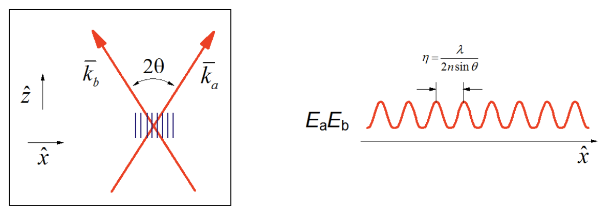
If the beams are crossed at an angle \(2\theta\)

\[\begin{aligned} \bar k_a &=|k_a|(\hat z\cos{\theta}+\hat x\sin{\theta}) \\ \bar k_b &=|k_b|(\hat z\cos{\theta}-\hat x\sin{\theta}) \end{aligned} \label{4.3.2}\]

with

\[|k_a|=|k_b|=\frac{2\pi n}{\lambda} \label{4.3.3}\]

the excitation of the sample is a spatial varying interference pattern along the transverse direction

\[\bar E_a \bar E_b=E_aE_b \exp[i\bar\beta\cdot\bar x]+c.c. \label{4.3.4}\]

The grating wavevector is

\[\begin{aligned} \bar\beta &=\bar k_1-\bar k_2 \\[4pt] |\bar\beta| &= \frac{4\pi n}{\lambda}\sin{\theta} =\frac{2\pi}{\eta} \end{aligned} \label{4.3.5}\]

This spatially varying field pattern is called a grating, and has a fringe spacing

\[\eta=\frac{\lambda}{2n\sin{\theta}} \label{4.3.6}\]

Absorption images this pattern into the sample, creating a spatial pattern of excited and ground state molecules. A time-delayed probe beam can scatter off this grating, where the wavevector matching conditions are equivalent to the constructive interference of scattered waves at the Bragg angle off a diffraction grating. For \(\omega_1=\omega_2=\omega_3=\omega_{sig}\) this the diffraction condition is incidence of \(\bar k_3\) at an angle \(\theta\), leading to scattering of a signal out of the sample at an angle \(-\theta\). Most commonly, we measure the intensity of the scattered light, as given in eq. (4.2.8)

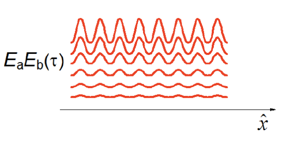
More generally, we should think of excitation with this pulse pair leading to a periodic spatial variation of the complex index of refraction of the medium. Absorption can create an excited state grating, whereas subsequent relaxation can lead to heating a periodic temperature profile (a thermal grating). Nonresonant scattering processes (Raleigh and Brillouin scattering) can create a spatial modulation in the real index or refraction. Thus, the transient grating signal will be sensitive to any processes which act to wash out the spatial modulation of the grating pattern:

• Population relaxation leads to a decrease in the grating amplitude, observed as a decrease in diffraction efficiency.

\[I_{sig}(\tau) \propto exp[-2\Gamma_{bb}\tau] \label{4.3.7}\]

• Thermal or mass diffusion along \(\hat x\) acts to wash out the fringe pattern. For a diffusion constant D the decay of diffraction efficiency is

\[I_{sig}(\tau)\propto exp[-2\beta^2D\tau] \label{4.3.8}\]

• Rapid heating by the excitation pulses can launch counter propagating acoustic waves along \(\hat x\), which can modulate the diffracted beam at a frequency dictated by the period for which sound propagates over the fringe spacing in the sample.