2.4: Example- Second-Order Response for a Three-Level System

Last updated
Save as PDF

Page ID: 303085

\( \newcommand{\vecs}[1]{\overset { \scriptstyle \rightharpoonup} {\mathbf{#1}} } \) \( \newcommand{\vecd}[1]{\overset{-\!-\!\rightharpoonup}{\vphantom{a}\smash {#1}}} \)\(\newcommand{\id}{\mathrm{id}}\) \( \newcommand{\Span}{\mathrm{span}}\) \( \newcommand{\kernel}{\mathrm{null}\,}\) \( \newcommand{\range}{\mathrm{range}\,}\) \( \newcommand{\RealPart}{\mathrm{Re}}\) \( \newcommand{\ImaginaryPart}{\mathrm{Im}}\) \( \newcommand{\Argument}{\mathrm{Arg}}\) \( \newcommand{\norm}[1]{\| #1 \|}\) \( \newcommand{\inner}[2]{\langle #1, #2 \rangle}\) \( \newcommand{\Span}{\mathrm{span}}\) \(\newcommand{\id}{\mathrm{id}}\) \( \newcommand{\Span}{\mathrm{span}}\) \( \newcommand{\kernel}{\mathrm{null}\,}\) \( \newcommand{\range}{\mathrm{range}\,}\) \( \newcommand{\RealPart}{\mathrm{Re}}\) \( \newcommand{\ImaginaryPart}{\mathrm{Im}}\) \( \newcommand{\Argument}{\mathrm{Arg}}\) \( \newcommand{\norm}[1]{\| #1 \|}\) \( \newcommand{\inner}[2]{\langle #1, #2 \rangle}\) \( \newcommand{\Span}{\mathrm{span}}\)\(\newcommand{\AA}{\unicode[.8,0]{x212B}}\)

The second-order response is the simplest nonlinear case, but in molecular spectroscopy is less commonly used than third-order measurements. The signal generation requires a lack of inversion symmetry, which makes it useful for studies of interfaces and chiral systems. However, let’s show how one would diagrammatically evaluate the second order response for a very specific system pictured below.

If we only have population in the ground state at equilibrium and if there are only resonant interactions allowed, the permutations of unique diagrams are as follows:

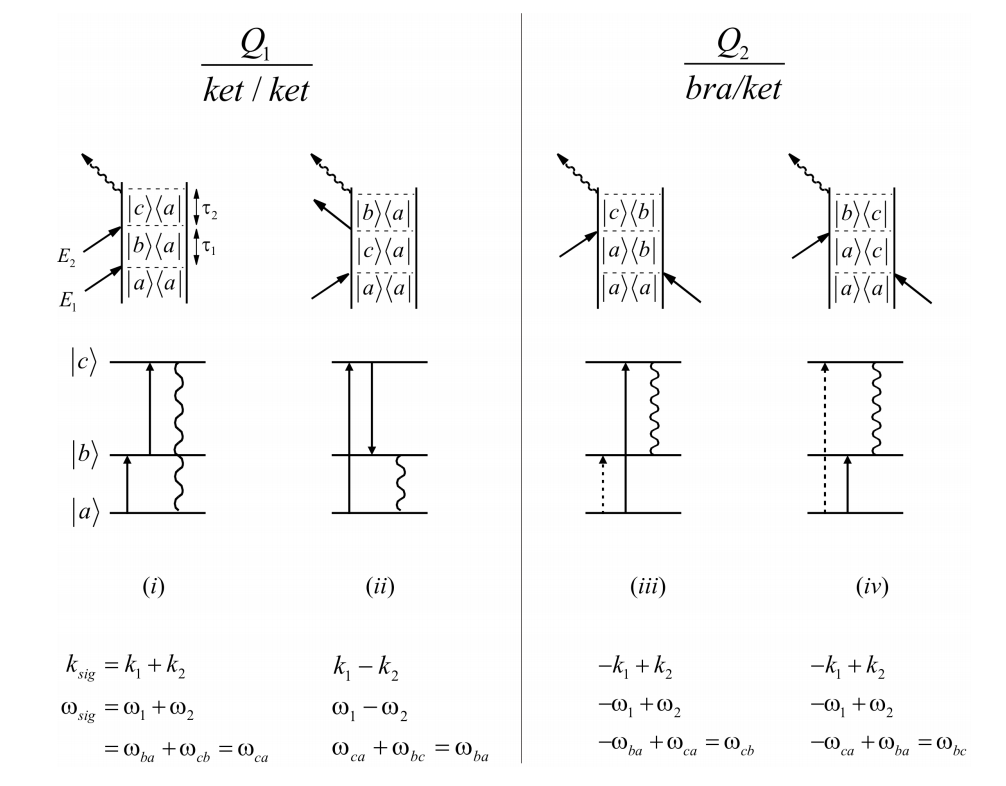
From the frequency conservation conditions, it should be clear that process i is a sum-frequency signal for the incident fields, whereas diagrams ii-iv refer to difference frequency schemes. To better interpret what these diagrams refer to let’s look at iii. Reading in a time-ordered manner, we can write the correlation function corresponding to this diagram as

\[\begin{aligned} C_{2} &=\operatorname{Tr}\left[\mu(\tau) \rho_{e q} \mu(0)\right] \\[4pt] &=(-1)^{1} \mu_{b c} \hat{G}_{c b}\left(\tau_{2}\right) \mu_{c a} \hat{G}_{a b}\left(\tau_{1}\right) \rho_{a a} \mu_{b a}^{*} \\[4pt] &=-p_{a} \mu_{a b} \mu_{b c} \mu_{c a} e^{-i \omega_{a b} \tau_{1}-\Gamma_{a b} \tau_{1}} e^{-i \omega_{c b} \tau_{2}-\Gamma_{c b} \tau_{2}} \end{aligned} \label{3.4.1}\]

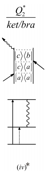
Note that a literal interpretation of the final trace in diagram iv would imply an absorption event – an upward transition from b to c. What does this have to do with radiating a signal? On the one hand it is important to remember that a diagram is just mathematical shorthand, and that one can’t distinguish absorption and emission in the final action of the dipole operator prior to taking a trace. The other thing to remember is that such a diagram always has a complex conjugate associated with it in the response function. The complex conjugate of iv, a \(Q_2^*\) ket/bra term, shown below has a downward transition –emission– as the final interaction. The combination \(Q_2 − Q_2^*\) ultimately describes the observable.

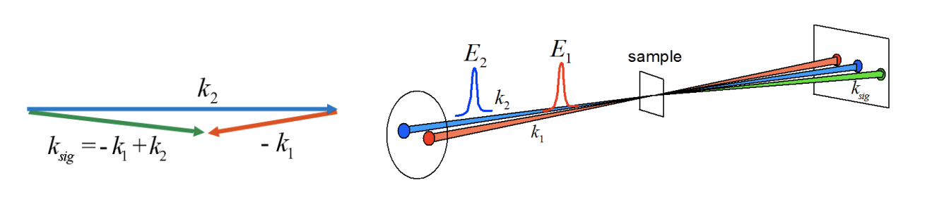
Now, consider the wavevector matching conditions for the second order signal iii. Remembering that the magnitude of the wavevector is \(|\bar k| = \omega/c = 2\pi / \lambda\), the length of the vectors will be scaled by the resonance frequencies. When the two incident fields are crossed as a slight angle, the signal would be phase-matched such that the signal is radiated closest to beam 2. Note that the most efficient wavevector matching here would be when fields 1 and 2 are collinear.