2.2: Ladder Diagrams

Ladder Diagrams¹ are helpful for describing experiments on multistate systems and/or with multiple frequencies; however, it is difficult to immediately see the state of the system during a given time interval. They naturally lend themselves to a description of interactions in terms of the eigenstates of \(H_0\).

1. Multiple states arranged vertically by energy.
2. Time propagates to right.
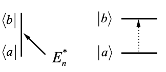
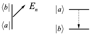
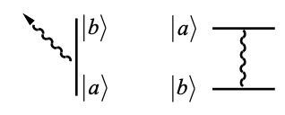
3. Arrows connecting levels indicate resonant interactions. Absorption is an upward arrow and emission is downward. A solid line is used to indicate action on the ket, whereas a dotted line is action on the bra.
4. Free propagation under \(H_0\) between interactions, but the state of the density matrix is not always obvious.

For each light-matter interactions represented in a diagram, there is an understanding of how this action contributes to the response function and the final nonlinear polarization state. Each light-matter interaction acts on one side of \(\rho\), either through absorption or stimulated emission. Each interaction adds a dipole matrix element \(\mu_{ij}\) that describes the interaction amplitude and any orientational effects.² Each interaction adds input electric field factors to the polarization, which are used to describe the frequency and wavevector of the radiated signal. The action of the final dipole operator must return you to a diagonal element to contribute to the signal. Remember that action on the bra is the complex conjugate of ket and absorption is complex conjugate of stimulated emission. A table summarizing these interactions contributing to a diagram is below

Interaction	Diagrammatic Representation	contrib. to \(R^{(n)}\)	contrib. to ksig & \(\omega_{sig}\)
KET SIDE Absorption \[(\bar\mu_{ba}\cdot\bar E_n)exp[i\bar k_n\cdot\bar r - i\omega_nt]\nonumber\]		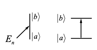\[\bar\mu_{ba}\cdot\hat\epsilon_n \nonumber\]	+kn \(+\omega_n\)
Stimulated Emission \[(\bar\mu_{ba}\cdot\bar E_n^*)exp[i\bar k_n\cdot\bar r - i\omega_nt]\nonumber\]		\[\bar\mu_{ba}\cdot\hat\epsilon_n \nonumber\]	-kn \(-\omega_n\)
BRA SIDE Absorption \[(\bar\mu_{ba}^*\cdot\bar E_n^*)exp[i\bar k_n\cdot\bar r - i\omega_nt]\nonumber\]		\[\bar\mu_{ba}^*\cdot\hat\epsilon_n \nonumber\]	-kn \(-\omega_n\)
Stimulated Emission \[(\bar\mu_{ba}^*\cdot\bar E_n)exp[i\bar k_n\cdot\bar r - i\omega_nt]\nonumber\]		\[\bar\mu_{ba}^*\cdot\hat\epsilon_n \nonumber\]	+kn \(+\omega_n\)
SIGNAL EMISSION (final trace, convention: ket side)		\[\bar\mu_{ba}\cdot\hat\epsilon_{an} \nonumber\]

Once you have written down the relevant diagrams, being careful to identify all permutations of interactions of your system states with the fields relevant to your signal, the correlation functions contributing to the material response and the frequency and wavevector of the signal field can be readily obtained. It is convenient to write the correlation function as a product of several factors for each event during the series of interactions:

1. Start with a factor \(p_n\) signifying the probability of occupying the initial state, typically a Boltzmann factor.
2. Read off products of transition dipole moments for interactions with the incident fields, and for the final signal emission.
3. Multiply by terms that describe the propagation under \(H_0\) between interactions. As a starting point for understanding an experiment, it is valuable to include the effects of relaxation of the system eigenstates in the time-evolution using a simple phenomenological approach. Coherences and populations are propagated by assigning the damping constant \(\Gamma_{ab}\) to propagation of the \(\rho_{ab}\) element:

\[\hat G(\tau)\rho_{ab}=exp[-i\omega_{ab}\tau-\Gamma_{ab}\tau]\rho_{ab}\]

Note \(\Gamma_{ab} = \Gamma_{ba}\) and \(G_{ab}^* = G_{ba}\). We can then recognize \(\Gamma_{ii}=1/T_1\) as the population relaxation rate for state i and \(\Gamma_{ij} = 1/T_2\) the dephasing rate for the coherence \(\rho_{ij}\).

4) Multiply by a factor of (−1)ⁿ where n is the number of bra side interactions. This factor accounts for the fact that in evaluating the nested commutator, some correlation functions are subtracted from others.

5) The radiated signal will have frequency \(\displaystyle\omega_{sig}=\sum_i\omega_i\) and wave vector \(\displaystyle\bar k_{sig}=\sum_i\bar k_i\)

1. D. Lee and A. C. Albrecht, “A unified view of Raman, resonance Raman, and fluorescence spectroscopy (and their analogues in two-photon absorption).” Adv. Infrared and Raman Spectr. 12, 179 (1985).

2. To properly account for all orientational factors, the transition dipole moment must be projected onto the incident electric field polarization \(\hat\epsilon\) leading to the terms in the table. This leads to a nonlinear polarization that can have x, y, and z polarization components in the lab frame. The are obtained by projecting the matrix element prior to the final trace onto the desired analyzer axis \(\hat\epsilon_{an}\).