
1: Coherent Spectroscopy and the Nonlinear Polarization
- Page ID
- 298948

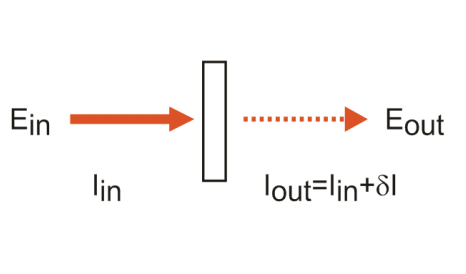
We will specifically be dealing with the description of coherent nonlinear spectroscopy, which is the term used to describe the case where one or more input fields coherently act on the dipoles of the sample to generate a macroscopic oscillating polarization. This polarization acts as a source to radiate a signal that we detect in a well-defined direction. This class includes experiments such as pump-probes, transient gratings, photon echoes, and coherent Raman methods. However understanding these experiments allows one to rather quickly generalize to other techniques.
| Detection: | Coherent | Spontaneous |
| \[ I_{coherent}\propto|\sum_i\mu_i|^2\nonumber\] | \[ I_{spont}\propto\sum_i|\mu_i|^2\nonumber\] | |
| Linear |
Absorption
|
Fluorescence, phosphorescence, Raman, and light scattering
|
| Nonlinear |
Pump-probe transient absorption, photon echoes, transient gratings, CARS, impulsive Raman scattering |
Fluorescence-detected nonlinear spectroscopy, i.e. stimulated emission pumping, time-dependent Stokes shift |
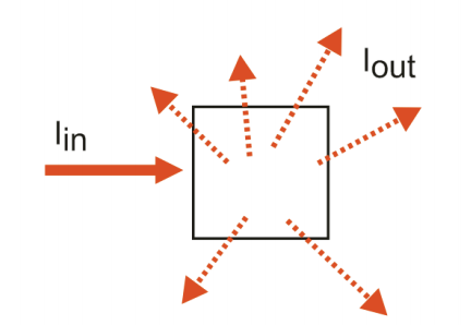
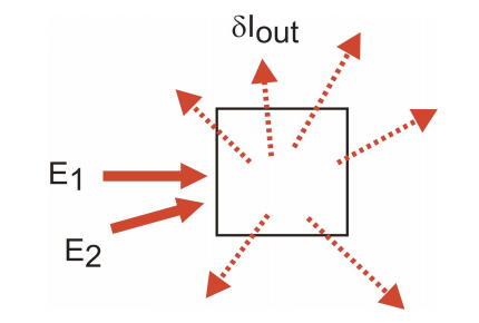
Spontaneous and coherent signals are both emitted from all samples, however, the relative amplitude of the two depend on the time-scale of dephasing within the sample. For electronic transitions in which dephasing is typically much faster than the radiative lifetime, spontaneous emission is the dominant emission process. For the case of vibrational transitions where non-radiative relaxation is typically a picoseconds process and radiative relaxation is a µs or longer process, spontaneous emission is not observed. The description of coherent nonlinear spectroscopies is rooted in the calculation of the polarization, P . The polarization is a macroscopic collective dipole moment per unit volume, and for a molecular system is expressed as a sum over the displacement of all charges for all molecules being interrogated by the light.
Sum over molecules:
\[\bar P (\bar r) = \sum_m \bar \mu_m \delta ( \bar r - \bar R_m) \]
Sum over charges on molecules:
\[\bar \mu_m \equiv \sum_{\alpha} q_{m\alpha} (\bar r_{m\alpha} - \bar R_m) \]
In coherent spectroscopies, the input fields E act to create a macroscopic, coherently oscillating charge distribution.
\[\bar P(\omega) = \chi \bar E (\omega) \]
as dictated by the susceptibility of the sample. The polarization acts as a source to radiate a new electromagnetic field, which we term the signal \(\bar E_{sig}\). (Remember that an accelerated charge radiates an electric field.) In the electric dipole approximation, the polarization is one term in the current and charge densities that you put into Maxwell’s equations.
From our earlier description of freely propagating electromagnetic waves, the wave equation for a transverse, plane wave was
\[\bar \nabla^2 \bar E(\bar r, t) - \frac{1}{c^2}\frac{\partial^2\bar E(\bar r, t)}{\partial t^2} = 0\]
which gave a solution for a sinusoidal oscillating field with frequency ω propagating in the direction of the wavevector k. In the present case, the polarization acts as a source − an accelerated charge − and we can write
\[\bar \nabla^2 \bar E(\bar r, t) - \frac{1}{c^2}\frac{\partial^2\bar E(\bar r, t)}{\partial t^2} = \frac{4\pi}{c^2}\frac{\partial^2\bar P(\bar r, t)}{\partial t^2}\]
The polarization can be described by solutions of the form
\[\bar P (\bar r,t) = P(t)exp(i \bar k_{sig}' \cdot \bar r -i\omega_{sig}t) + c.c.\]
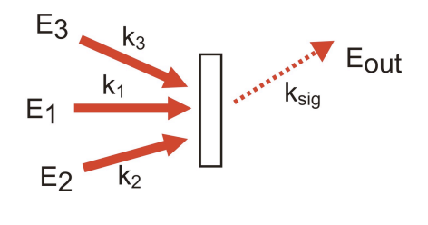
As we will discuss further later, the wavevector and frequency of the polarization depend on the frequency and wave vector of incident fields.
\[\bar k_{sig} = \sum_n\pm \bar k_n\]
\[\omega_{sig} = \sum_n\pm \omega_n\]
These relationships enforce momentum and energy conservation for the problem. The oscillating polarization radiates a coherent signal field, \(\bar E_{sig}\), in a wave vector matched direction \(\bar k_{sig}\). Although a single dipole radiates as a sinθ field distribution relative to the displacement of the charge,1 for an ensemble of dipoles that have been coherently driven by external fields, P is given by (2.6) and the radiation of the ensemble only constructively adds along \(\bar k_{sig}\). For the radiated field we obtain
\[\bar E_{sig} (\bar r,t) = E_{sig}(\bar r,t)exp(i \bar k_{sig} \cdot \bar r -i\omega_{sig}t) + c.c.\]
This solution comes from solving (2.5) for a thin sample of length l, for which the radiated signal amplitude grows and becomes directional as it propagates through the sample. The emitted signal
\[\bar E_{sig}(t) = i\frac{2\pi\omega_s}{nc}l \bar P(t)sinc(\frac{\Delta kl}{2})e^{i\Delta kl/2} \]
Here we note the oscillating polarization is proportional to the signal field, although there is a π/2 phase shift between the two, \(\bar E_{sig}\propto i \bar P\), because in the sample the polarization is related to the gradient of the field. Δk is the wave-vector mismatch between the wavevector of the polarization \(\bar k_{sig}'\) and the radiated field \(\bar k_{sig}\), which we will discuss more later.
For the purpose of our work, we obtain the polarization from the expectation value of the dipole operator
\[\bar P(t) \Rightarrow \bar{\mu(t)}\]
The treatment we will use for the spectroscopy is semi-classical, and follows the formalism that was popularized by Mukamel.2 As before, our Hamiltonian can generally be written as
\[H = H_0 + V(t)\]
where the material system is described by H0 and treated quantum mechanically, and the electromagnetic fields V(t) are treated classically and take the standard form
\[V(t)=-\bar \mu \cdot \bar E\]
The fields only act to drive transitions between quantum states of the system. We take the interaction with the fields to be sufficiently weak that we can treat the problem with perturbation theory. Thus, nth-order perturbation theory will be used to describe the nonlinear signal derived from interacting with n electromagnetic fields.
- The radiation pattern in the far field for the electric field emitted by a dipole aligned along the z axis is
\[E(r,\theta,\phi,t)=-\frac{p_0k^2}{4\pi\epsilon_0}\frac{\sin \theta}{r}\sin{(k \cdot r - \omega t)}\]
(written in spherical coordinates). See Jackson, Classical Electrodynamics. - S. Mukamel, Principles of Nonlinear Optical Spectroscopy. (Oxford University Press, New York, 1995).