
12.3: The Wave Equation in One Dimension
- Page ID
- 106878

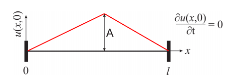
The wave equation is an important second-order linear partial differential equation that describes waves such as sound waves, light waves and water waves. In this course, we will focus on oscillations in one dimension. Let’s consider a thin string of length \(l\) that is fixed at its two endpoints, and let’s call the displacement of the string from its horizontal position \(u(x,t)\) (figure [fig:pde1]). The displacement of each point in the string is limited to one dimension, but because the displacement also depends on time, the one-dimensional wave equation is a PDE:
\[\label{eq:pde10} \dfrac{\partial^2u(x,t)}{\partial x^2}=\dfrac{1}{v^2}\dfrac{\partial^2 u(x,t)}{\partial t^2}\]
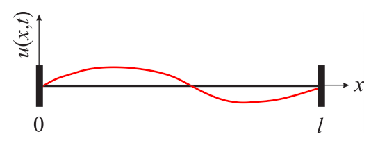
Because the string is held at both ends, the PDE is subject to two boundary conditions:
\[\label{eq:pde11} u(0,t)=u(l,t)=0\]
Using the method of separation of variables, we assume that the function \(u(x,t)\) can be written as the product of a function of only \(x\) and a function of only \(t\).
\[\label{eq:pde12} u(x,t)=f(x)g(t)\]
Substituting Equation \ref{eq:pde12} in Equation \ref{eq:pde10}:
\[\dfrac{\partial^2f(x)g(t)}{\partial x^2}=\dfrac{1}{v^2}\dfrac{\partial^2 f(x)g(t)}{\partial t^2} \nonumber\]
\[\label{eq:pde13} g(t)\dfrac{\partial^2 f(x)}{\partial x^2}=\dfrac{1}{v^2}f(x)\dfrac{\partial^2 g(t)}{\partial t^2}\]
and separating the terms in \(x\) from the terms in \(y\):
\[\label{eq:pde14} \dfrac{1}{f(x)}\dfrac{\partial^2 f(x)}{\partial x^2}=\dfrac{1}{v^2}\dfrac{1}{g(t)}\dfrac{\partial^2 g(t)}{\partial t^2}\]
Remember that \(v\) is a constant, and we could leave it on either side of Equation \ref{eq:pde14}. The left side of this equation is a function of \(x\) only, and the right side is a function of \(t\) only. Because \(x\) and \(t\) are independent variables, the only way that the equality holds is that each side equals a constant.
\[\dfrac{1}{f(x)}\dfrac{\partial^2 f(x)}{\partial x^2}=\dfrac{1}{v^2}\dfrac{1}{g(t)}\dfrac{\partial^2 g(t)}{\partial t^2}=K \nonumber\]
\(K\) is called the separation constant, and will be determined by the boundary conditions. Note that after separation of variables, one PDE became two ODEs:
\[\label{eq:pde15a} \dfrac{1}{f(x)}\dfrac{\partial^2 f(x)}{\partial x^2}=K\rightarrow \dfrac{\partial^2 f(x)}{\partial x^2}-Kf(x)=0\]
\[\label{eq:pde15b} \dfrac{1}{v^2}\dfrac{1}{g(t)}\dfrac{\partial^2 g(t)}{\partial t^2}=K\rightarrow \dfrac{\partial^2 g(t)}{\partial t^2}-Kv^2g(t)=0\]
These are both second order ordinary differential equations with constant coefficients, so we can solve them using the methods we learned in Chapter 5.
From Equation \ref{eq:pde15a},
\[\dfrac{\partial ^2f(x)}{\partial x^2}-Kf(x)=0 \nonumber\]
which is a 2nd order ODE with auxiliary equation
\[\alpha^2-K=0\Rightarrow \alpha=\pm\sqrt{K} \nonumber\]
and therefore
\[\label{eq:pde16} f(x)=c_1e^{\sqrt{K}x}+c_2e^{-\sqrt{K}x}\]
We do not know yet if \(K\) is positive, negative or zero, so we do not know if these are real or complex exponentials. We will use the boundary conditions (\(f(0)=f(l)=0\)) and see what happens:
\[f(x)=c_1e^{\sqrt{K}x}+c_2e^{-\sqrt{K}x}\rightarrow f(0)=c_1+c_2=0\Rightarrow c_1=-c_2 \nonumber\]
\[f(x)=c_1(e^{\sqrt{K}x}-e^{-\sqrt{K}x})\rightarrow f(l)=c_1(e^{\sqrt{K}l}-e^{-\sqrt{K}l})=0 \nonumber\]
There are two ways to make
\[f(l)=c_1(e^{\sqrt{K}l}-e^{-\sqrt{K}l})=0. \nonumber\]
We could choose \(c_1=0\), but this choice would result in \(f(x)=0\), which physically means the string is not vibrating at all (the displacement of all points is zero). This is certainly a mathematically acceptable solution, but it is not a solution that represents the physical behavior of our string. Therefore, the only viable choice is \(e^{\sqrt{K}l}=e^{-\sqrt{K}l}\). Let’s see what this means in terms of \(K\). There is no positive value of \(K\) that makes
\[e^{\sqrt{K}l}=e^{-\sqrt{K}l}. \nonumber\]
If \(K=0\), we obtain \(f(x)=0\), which is again not physically acceptable. Then, the value of \(K\) has to be negative, and \(\sqrt{K}\) is an imaginary number:
\[e^{\sqrt{K}l}=e^{-\sqrt{K}l} \nonumber\]
\[e^{i\sqrt{|K|}l}=e^{-i\sqrt{|K|}l} \nonumber\]
where \(|K|=-K\) is the absolute value of \(K<0\). Using Euler’s relationship:
\[\cos(\sqrt{|K|}l)+i\sin(\sqrt{|K|}l)=\cos(\sqrt{|K|}l)-i\sin(\sqrt{|K|}l) \nonumber\]
\[2i\sin(\sqrt{|K|}l)=0\rightarrow \sqrt{|K|}l=n\pi\rightarrow \sqrt{|K|}=\left( \dfrac{n\pi}{l}\right) \nonumber\]
Now that we have an expression for \(K\), we can write an expression for \(f(x)\):
\[f(x)=c_1(e^{\sqrt{K}x}-e^{-\sqrt{K}x})=c_1(e^{i\sqrt{|K|}x}-e^{-i\sqrt{|K|}x})=2ic_1\sin(\sqrt{|K|}x) \nonumber\]
\[\label{eq:pde17} f(x)=A\sin\left(\dfrac{n\pi}{l}x\right)\]
So far we got \(f(x)\), so we need to move on and get an expression for \(g(t)\) from Equation \ref{eq:pde15b}. Notice, however, that we now know the value of \(K\), so let’s re-write Equation \ref{eq:pde15b} as:
\[\label{eq:pde 18} \dfrac{\partial^2 g(t)}{\partial t^2}+\left(\dfrac{n\pi}{l}\right)^2v^2g(t)=0\]
This is another 2nd order ODE, with auxiliary equation
\[\alpha^2+\left(\dfrac{n\pi}{l}\right)^2v^2=0\rightarrow \alpha=\pm i \left( \dfrac{n\pi}{l} v\right) \nonumber\]
we can then write \(g(t)\) as:
\[g(t)=c_1e^{i \left( \dfrac{n\pi}{l} v\right) t}+c_2e^{-i \left( \dfrac{n\pi}{l} v\right) t} \nonumber\]
which you should be able to prove can be rewritten as
\[\label{eq:pde_19} g(t)=c_3\sin \left( \dfrac{n\pi}{l} vt\right) +c_4\cos \left( \dfrac{n\pi}{l} vt\right)\]
We cannot get the values of \(c_3\) and \(c_4\) yet because we do not have information about initial conditions. Before discussing this, however, let’s put the two pieces together:
\[u(x,t)=\sin \left( \dfrac{n\pi}{l}x \right) \left[p_n\sin \left( \dfrac{n\pi}{l} vt\right) +q_n\cos \left( \dfrac{n\pi}{l} vt\right) \right] \nonumber\]
where we combined the constants \(A\) and \(c_{1,2}\) and re-named them \(p_n\) and \(q_n\). The subindices stress the fact that these constants depend on \(n\), which will be important in a minute. Before we move on, and to simplify notation, let’s recognize that the quantity \(\dfrac{n \pi v}{l}\) has units of reciprocal time. This is true because it needs to give an dimensionless number when multiplied by \(t\). This means that, physically, \(\dfrac{n \pi v}{l}\) represents a frequency, so we can call it \(\omega_n\):
\[\label{eq:pde_20} u(x,t)=\sin \left( \dfrac{n\pi}{l}x \right) \left[p_n\sin \left(\omega_nt\right) +q_n\cos \left(\omega_nt\right) \right]\;n=1,2,...,\infty\]
At this point, we recognize that we have an infinite number of solutions:
\[\label{eq:pde_21} u_1(x,t)=\sin \left( \dfrac{\pi}{l}x \right) \left[p_1\sin \left(\omega_1t\right) +q_1\cos \left(\omega_1 t\right) \right]\]
\[u_2(x,t)=\sin \left( 2\dfrac{\pi}{l}x \right) \left[p_2\sin \left(\omega_2t\right) +q_2\cos \left(\omega_2t\right) \right] \nonumber\]
\[\vdots \nonumber\]
\[u_n(x,t)=\sin \left( n\dfrac{\pi}{l}x \right) \left[p_n\sin \left(\omega_nt\right) +q_n\cos \left(\omega_nt\right) \right] \nonumber\]
where \(\omega_1, \omega_2,...,\omega_n=\dfrac{\pi v}{l},\dfrac{2\pi v}{l},...,\dfrac{n\pi v}{l}\). As usual, the general solution is a linear combination of all these solutions:
\[\label{eq:pde_22} u(x,t)=c_1u_1(x,t)+c_2u_2(x,t)+...+c_nu_n(x,t)={\color{red}\sum_{n=1}^{\infty}\sin \left( \dfrac{n\pi}{l}x \right) \left[a_n\sin \left(\omega_nt\right) +b_n\cos \left(\omega_nt\right) \right]}\]
where \(a_n=c_np_n\) and \(b_n=c_nq_n\).
Notice that we have not used any initial conditions yet. We used the boundary conditions we were given (\(u(0,t)=u(l,t)=0\)), so Equation \ref{eq:pde_22} is valid regardless of initial conditions as long as the string is held fixed at both ends. As you may suspect, the values of \(a_n\) and \(b_n\) will be calculated from the initial conditions. However, notice that in order to describe the movement of the string at all times we will need to calculate an infinite number of \(a_n\)-values and and infinite number of \(b_n\)-values. This sounds pretty intimidating, but you will see how all the time you spent learning about Fourier series will finally pay off. Before we look into how to do that, let’s take a look at the individual solutions listed in Equation \ref{eq:pde_21}.
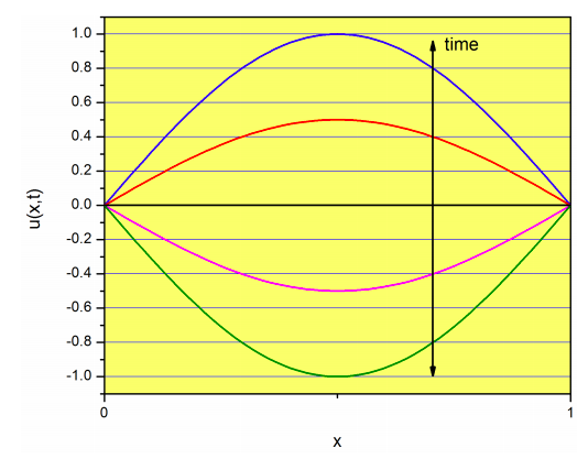
Each \(u_n(x,t)\) is called a normal mode. For example, for \(n=1\), we have
\[u_1(x,t)=\sin \left( \dfrac{\pi}{l}x \right) \left[p_1\sin \left(\omega_1t\right) +q_1\cos \left(\omega_1t\right) \right] \nonumber\]
which is called the fundamental mode, or first harmonic.
Notice that this function is the product of a function that depends only on \(x\) (\(\sin \left( \dfrac{\pi}{l}x \right)\) ) and another function that depends only on \(t\), i.e.,
\[\left[p_1\sin \left(\omega_1t\right) +q_1\cos \left(\omega_1t\right) \right]. \nonumber\]
The function on \(t\) simply changes the amplitude of the sine function on \(x\):
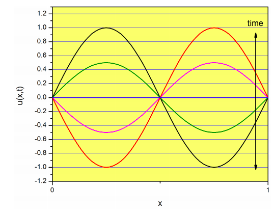
For \(n=2\), we have:
\[u_2(x,t)=\sin \left( 2\dfrac{\pi}{l}x \right) \left[p_2\sin \left(\omega_2t\right) +q_2\cos \left(\omega_2t\right) \right] \nonumber\]
which is called the first overtone, or second harmonic. Again, this function is the product of one function that depends on \(x\) only (\(\sin \left( 2\dfrac{\pi}{l}x \right)\)), and another one that depends on \(t\) and changes the amplitude of \(\sin \left( 2\dfrac{\pi}{l}x \right)\) without changing its overall shape:
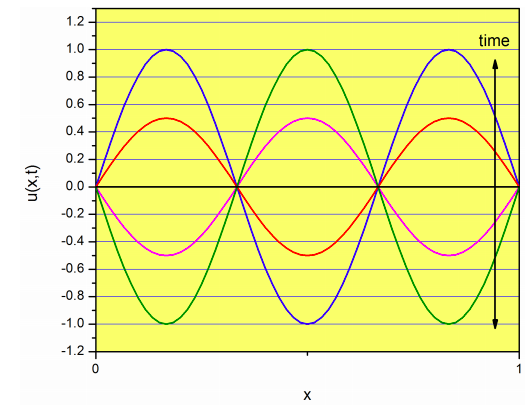
For \(n=3\), we have:
\[u_3(x,t)=\sin \left( 3\dfrac{\pi}{l}x \right) \left[p_3\sin \left(\omega_3t\right) +q_3\cos \left(\omega_3t\right) \right] \nonumber\]
which is called the second overtone, or third harmonic. Again, this function is the product of one function that depends on \(x\) only (\(\sin \left( 3\dfrac{\pi}{l}x \right)\)), and another one that depends on \(t\) and changes the amplitude of \(\sin \left( 3\dfrac{\pi}{l}x \right)\) without changing its overall shape:
If the initial shape of the string (i.e. the function \(u(x,t)\) at time zero) is \(\sin \left( \dfrac{\pi}{l}x \right)\) (Figure \(\PageIndex{2}\), then the string will vibrate as shown in the figure, just changing the amplitude but not the overall shape. In more general terms, if \(u(x,0)\) is one of the normal modes, the string will vibrate according to that normal mode, without mixing with the rest. However, in general, the shape of the string will be described by a linear combination of normal modes (Equation \ref{eq:pde_22}). If you recall from Chapter 7, a Fourier series tells you how to express a function as a linear combination of sines and cosines. The idea here is the same: we will express an arbitrary shape as a linear combination of normal modes, which are a collection of sine functions.
In order to do that, we need information about the initial shape: \(u(x,0)\). We also need information about the initial velocity of all the points in the string: \(\dfrac{\partial u(x,0)}{\partial t}\). The initial shape is the displacement of all points at time zero, and it is a function of \(x\). Let’s call this function \(y_1(x)\):
\[\label{eq:pde23} u(x,0)=y_1(x)\]
The initial velocity of all points is also a function of \(x\), and we will call it \(y_2(x)\):
\[\label{eq:pde24} \dfrac{\partial u(x,0)}{\partial t}=y_2(x)\]
Both functions together represent the initial conditions, and be will used to calculate all the \(a_n\) and \(b_n\) coefficients. To simplify the problem, let’s assume that at time zero we hold the string still, so the velocity of all points is zero:
\[\dfrac{\partial u(x,0)}{\partial t}=0 \nonumber\]
Let’s see how we can use this information to finish the problem (i.e. calculate the coefficients \(a_n\) and \(b_n\)). From Equations \ref{eq:pde_22} and \ref{eq:pde23}:
\[u(x,t)=\sum_{n=1}^{\infty}\sin \left( \dfrac{n\pi}{l}x \right) \left[a_n\sin \left(\omega_nt\right) +b_n\cos \left(\omega_nt\right) \right] \nonumber\]
and applying the first initial condition:
\[\label{eq:pde_25} u(x,0)=\sum_{n=1}^{\infty}\sin \left( \dfrac{n\pi}{l}x \right) [b_n]=y_1(x)\]
This equation tells us that the initial shape, \(y_1(x)\), can be described as an infinite sum of sine functions....sounds familiar? In Chapter 7, we saw that we can represent a periodic odd function \(f(x)\) of period \(2L\) as an infinite sum of sine functions (Equation \(7.2.1\), \( f(x)=\dfrac{a_0}{2}+\sum_{n=1}^{\infty}a_n \cos\left ( \dfrac{n\pi x}{L} \right )+\sum_{n=1}^{\infty}b_n \sin\left ( \dfrac{n\pi x}{L} \right )\) ):
\[\label{eq:pde_26} f(x)=\sum_{n=1}^{\infty}b_n sin\left ( \dfrac{n\pi x}{L} \right )\]
Comparing Equations \ref{eq:pde_25} and \ref{eq:pde_26}, we see that in order to calculate the \(b_n\) coefficients of Equation \ref{eq:pde_22}, we need to create an odd extension of \(y_1\) with period \(2l\).
Let’s see how this works with an example. Let’s assume that the initial displacement is given by the function shown in the figure:
Equation \ref{eq:pde_25} tells us that the function of Figure \(\PageIndex{5}\) can be expressed as an infinite sum of sine functions. If we figure out which sum, we will have the coefficients \(b_n\) we need to write down the expression of \(u(x,y)\) we are seeking (Equation \ref{eq:pde_22}). We will still need the coefficients \(a_n\), which will be calculated from the second initial condition (Equation \ref{eq:pde24}).
Because we know the infinite sum of Equation \ref{eq:pde_25} describes an odd periodic function of period \(2l\), our first step is to extend \(y_1(x)\) in an odd fashion:
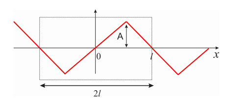
What is the Fourier series of the periodic function of Figure \(\PageIndex{6}\)? Using the methods we learned in Chapter 7, we obtain:
\[\label{eq:pde_27} y_1(x)=\dfrac{8A}{\pi^2}\left[\sin \dfrac{\pi x}{l}- \dfrac{1}{3^2}\sin\dfrac{3\pi x}{l} + \dfrac{1}{5^2}\sin\dfrac{5\pi x}{l}... \right]=\dfrac{8A}{\pi^2} \sum\limits_{n=0}^{\infty}\dfrac{(-1)^n}{(2n+1)^2} \sin \left( \dfrac{(2n+1)\pi}{l}x \right)\]
From Equation \ref{eq:pde_25}
\(u(x,0)=\sum\limits_{n=1}^{\infty}\sin \left( \dfrac{n\pi}{l}x \right) [b_n]=y_1(x)\)
comparing Equations \ref{eq:pde_25} and \ref{eq:pde_27}:
\[\label{eq:pde_28} b_n = \begin{cases} 0& n=2,4,6... \\ \dfrac{8A}{\pi^2n^2} & n=1,5,9... \\ - \dfrac{8A}{\pi^2n^2} & n=3,7,11... \end{cases}\]
Great! we have all the coefficients \(b_n\), so we are just one step away from our final goal of expressing \(u(x,t)\). Our last step is to calculate the coefficients \(a_n\). We will use the last initial condition: \(\dfrac{\partial u(x,0)}{\partial t}=y_2(x)\). Taking the partial derivative of Equation \ref{eq:pde_22}:
\[u(x,t)=\sum\limits_{n=1}^{\infty}\sin \left( \dfrac{n\pi}{l}x \right) \left[a_n\sin \left(\omega_nt\right) +b_n\cos \left(\omega_nt\right) \right] \nonumber\]
\[\dfrac{\partial u(x,t)}{\partial t}=\sum\limits_{n=1}^{\infty}\sin \left( \dfrac{n\pi}{l}x \right) \left[a_n\omega_n\cos \left(\omega_nt\right) -b_n\omega_n\sin \left(\omega_nt\right) \right] \nonumber\]
\[\label{eq:pde_29} \dfrac{\partial u(x,0)}{\partial t}=\sum\limits_{n=1}^{\infty}\sin \left( \dfrac{n\pi}{l}x \right) \left[a_n\omega_n\right]=y_2(x)\]
Equation \ref{eq:pde_29} tells us that the function \(y_2(x)\) can be expressed as an infinite sum of sine functions. Again, we need to create an odd extension of \(y_2(x)\) and obtain its Fourier series: \(y_2(x)=\sum_{n=1}^{\infty}b_n sin\left ( \dfrac{n\pi x}{L} \right )\). The coefficients \(b_n\) of the Fourier series equal \(a_n\omega_n\) (Equation \ref{eq:pde_29}). In this particular case:
\[\dfrac{\partial u(x,0)}{\partial t}=\sum\limits_{n=1}^{\infty}\sin \left( \dfrac{n\pi}{l}x \right) \left[a_n\omega_n\right]=0\rightarrow a_n=0 \nonumber\]
The coefficients \(a_n\) are zero, because the derivative needs to be zero for all values of \(x\).
Now that we have all coefficients \(b_n\) and \(a_n\) we are ready to wrap this up. From Equations \ref{eq:pde_22} and \ref{eq:pde_28}:
\[\begin{align} u(x,t) &=\sum\limits_{n=1}^{\infty}\sin \left( \dfrac{n\pi}{l}x \right) \left[a_n\sin \left(\omega_nt\right) +b_n\cos \left(\omega_nt\right) \right] \\[4pt] &=b_1\sin \left( \dfrac{\pi}{l}x \right)\cos \left( \omega_1t \right)+b_3\sin \left( \dfrac{3\pi}{l}x \right)\cos \left( \omega_3t \right)+b_5\sin \left( \dfrac{5\pi}{l}x \right)\cos \left( \omega_5t \right)... \\[4pt] &=\dfrac{8A}{\pi^2}\left[\sin \left( \dfrac{\pi}{l}x \right)\cos \left( \omega_1t \right)-\dfrac{1}{3^2}\sin \left( \dfrac{3\pi}{l}x \right)\cos \left( \omega_3t \right)+\dfrac{1}{5^2}\sin \left( \dfrac{5\pi}{l}x \right)\cos \left( \omega_5t \right)...\right] \end{align} \nonumber\]
Recalling that \(\omega_n=\dfrac{n\pi}{l}v\):
\[u(x,t)=\dfrac{8A}{\pi^2}\left[\sin \left( \dfrac{\pi}{l}x \right)\cos \left( \dfrac{\pi }{l}vt \right)-\dfrac{1}{3^2}\sin \left( \dfrac{3\pi}{l}x \right)\cos \left( \dfrac{3\pi }{l}vt \right)+\dfrac{1}{5^2}\sin \left( \dfrac{5\pi}{l}x \right)\cos \left(\dfrac{5\pi }{l}vt \right)...\right] \nonumber\]
\[\label{eq:pde_30} {\color{Maroon}u(x,t)=\dfrac{8A}{\pi^2}\sum\limits_{n=0}^{\infty}\dfrac{(-1)^n}{(2n+1)^2}\sin \left( \dfrac{(2n+1)\pi}{l}x \right) \cos \left(\dfrac{(2n+1)\pi }{l}vt \right)}\]
Success! We got a full description of the movement of the string. We just need to know the length of the string (\(l\)), the initial displacement of the midpoint (\(A\)) and the parameter \(v\), and we can start plotting the shape of the string at different times. Just remember that Mathematica cannot plot a function defined as an infinite sum, so you will have to plot a truncated version of Equation \ref{eq:pde_30}. As usual, the more terms you include the better the approximation, but the longer the computer will take to execute the command. To see an amazing slow motion movie of a real string follow this youtube link.
The parameter \(v\) has units of length over time (e.g. m/s), and it depends on factors such as the material of the string, its tension, and its thickness. A string instrument like a guitar, for instance, has strings made of different materials, and held at different tensions. When plucked, they produce vibrations of different frequencies, which we perceive as different musical notes. In general, the vibration of the string will be a linear combination of the normal modes we talked about earlier in this section. Each normal mode has a unique frequency (\(\omega_n=\dfrac{n\pi}{l}v\)), and if this frequency is within our audible range, we will perceive it as a pure musical note. A linear combination of normal modes contains many frequencies, and we perceive them as a more complex sound.
Music is nice, but what about the applications of normal modes in chemistry? We already mentioned molecular vibrations in different chapters, and we know that the atoms in molecules are continuously vibrating following approximately harmonic motions. The same way that the vibration of the string of Figure \(\PageIndex{5}\) can be expressed as a linear combination of all the normal modes (Figures \(\PageIndex{2}\)-\(\PageIndex{4}\), we can express the vibrations of a polyatomic molecule as a linear combination of normal modes. As you will see in your advanced physical chemistry courses, a non-linear polyatomic molecule has \(3n-6\) vibrational normal modes, where \(n\) is the number of atoms. For the molecule of water, for example, we have 3 normal modes:
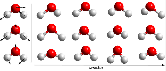
Any other type of vibration can be expressed as a linear combination of these three normal modes. As you can imagine, these motions occur very fast. Typically, you may see of the order of \(10^{12}\) vibrations per second. The most direct way of probing the vibrations of a molecule is through infra-red spectroscopy, and in fact you will measure and analyze the vibrational spectra of simple molecules in your 300-level physical chemistry labs.