
10.4: A Brief Introduction to Probability
- Page ID
- 106865

We have talked about the fact that the wavefunction can be interpreted as a probability, but this is a good time to formalize some concepts and understand what we really mean by that.
Let’s start by reviewing (or learning) a few concepts in probability theory. First, a random variable is a variable whose value is subject to variations due to chance. For example, we could define a variable that equals the number of days that it rains in Phoenix every month, or the outcome of throwing a die (the number of dots facing up), or the time it takes for the next bus to arrive to the bus station, or the waiting time we will have to endure next time we call a customer service phone line. Some of these random variables are discrete; the number of rain days or the number of dots facing up in a die can take on only a countable number of distinct values. For the case of the die, the outcome can only be \(\{1,2,3,4,5,6\}\). In contrast, a waiting time is a continuous random variable. If you could measure with enough precision, the random variable can take any positive real value. Coming back to physical chemistry, the position of an electron in an atom or molecule is a good example of a continuous random variable.
Imagine a (admittedly silly) game that involves flipping two coins. You get one point for each tail, and two points for each head. The game has three possible outcomes: 2 points (if you get two tails), 3 points (if you get one tail and one head) and 4 points (if you get two heads). The outcomes do not have the same probability. The probability of getting two heads or two tails is 1/4, while the probability that you get one head and one tail is 1/2. If we define a random variable (\(x\)) that equals the number of points you get in one round of the game, we can represent the probabilities of getting each possible outcome as:
| \(x\) | 2 | 3 | 4 |
|---|---|---|---|
| \(P(x)\) | 1/4 | 1/2 | 1/4 |
The collection of outcomes is called the sample space. In this case, the sample space is \(\{2,3,4\}\). If we add \(P(x)\) over the sample space we get, as expected, 1. In other words, the probability that you get an outcome that belongs to the sample space needs to be 1, which makes sense because we defined the sample space as the collection of all possible outcomes. If you think about an electron in an atom, and define the position in polar coordinates, \(r\) (the distance from the nucleus of the atom) is a random variable that can take any value from 0 to \(\infty\). The sample space for the random variable \(r\) is the set of positive real numbers.
Coming back to our discrete variable \(x\), our previous argument translates into
\[\sum\limits_{sample\; space}P(x)=1 \nonumber\]
Can we measure probabilities? Not exactly, but we can measure the frequency of each outcome if we repeat the experiment a large number of times. For example, if we play this game three times, we do not know how many times we’ll get 2, 3 or 4 points. But if we play the game a very large number of times, we know that half the time we will get 3 points, a quarter of the time will get 2 points, and another quarter 4 points. The probability is the frequency of an outcome in the limit of an infinite number of trials. Formally, the frequency is defined as the number of times you obtain a given outcome divided for the total number of trials.
Now, even if we do not have any way of predicting the outcome of our random experiment (the silly game we described above), if you had to bet, you would not think it twice and bet on \(x=3\) (one head and one tail). The fact that a random variable does not have a predictable outcome does not mean we do not have information about the distribution of probabilities. Coming back to our atom, we will be able to predict the value of \(r\) at which the probability of finding the electron is highest, the average value of \(r\), etc. Even if we know that \(r\) can take values up to \(\infty\), we know that it is much more likely to find it very close to the nucleus (e.g. within an angstrom) than far away (e.g. one inch). No physical law forbids the electron to be 1 inch from the nucleus, but the probability of that happening is so tiny, that we do not even think about this possibility.
The Mean of a Discrete Distribution
Let’s talk about the mean (or average) some more. What is exactly the average of a random variable? Coming back to our “game”, it would be the average value of \(x\) you would get if you could play the game an infinite number of times. You could also ask the whole planet to play the game once, and that would accomplish the same. The planet does not have an infinite number of people, but the average you get with several billion trials of the random experiment (throwing two coins) should be pretty close to the real average. We will denote the average (also called the mean) with angular brackets: \(\left \langle x \right \rangle\). Let’s say that we play this game \(10^9\) times. We expect 3 points half the time (frequency = \(1/2\)), or in this case, \(5\times 10^8\) times. We also expect 2 points or 4 points with a frequency of \(1/4\), so in this case, \(2.5 \times 10^8\) times. What is the average?
\[\left \langle x \right \rangle=\dfrac{1}{4}\times 2+\dfrac{1}{2}\times 3+\dfrac{1}{4}\times 4=3 \nonumber\]
On average, the billion people playing the game (or you playing it a billion times) should get 3 points. This happens to be the most probable outcome, but it does not need to be the case. For instance, if you just flip one coin, you can get 1 point or 2 points with equal probability, and the average will be 1.5, which is not the most probable outcome. In fact, it is not even a possible outcome!.
In general, it should make sense that for a discrete variable:
\[\label{eq:mean_discrete} \left \langle x \right \rangle=\sum\limits_{i=1}^k P(x_i)x_i\]
where the sum is performed over the whole sample space, which contains \(k\) elements. Here, \(x_i\) is each possible outcome, and \(P(x_i)\) is the probability of obtaining that outcome (or the fraction of times you would obtain it if you were to perform a huge number of trials).
Continuous Variables
How do we translate everything we just said to a continuous variable? As an example, let’s come back to the random variable \(r\), which is defined as the distance of the electron in the hydrogen atom from its nucleus. As we will see shortly, the 1s electron in the hydrogen atom spends most of its time within a couple of angstroms from the nucleus. We may ask ourselves, what is the probability that the electron will be found exactly at 1Å from the nucleus? Mathematically, what is \(P(r=1\) Å)? The answer will disappoint you, but this probability is zero, and it is zero for any value of \(r\). The electron needs to be somewhere, but the probability of finding it an any particular value of \(r\) is zero? Yes, that is precisely the case, and it is a consequence of \(r\) being a continuous variable. Imagine that you get a random real number in the interval [0,1] (you could do this even in your calculator), and I ask you what is the probability that you get exactly \(\pi/4\). There are infinite real numbers in this interval, and all of them are equally probable, so the probability of getting each of them is \(1/\infty=0\). Talking about the probabilities of particular outcomes is not very useful in the context of continuous variables. All the outcomes have a probability of zero, even if we intuitively know that the probability of finding the electron within 1Å is much larger than the probability of finding it at several miles. Instead, we will talk about the density of probability (\(p(r)\)). If you are confused about why the probability of a particular outcome is zero check the video listed at the end of this section.
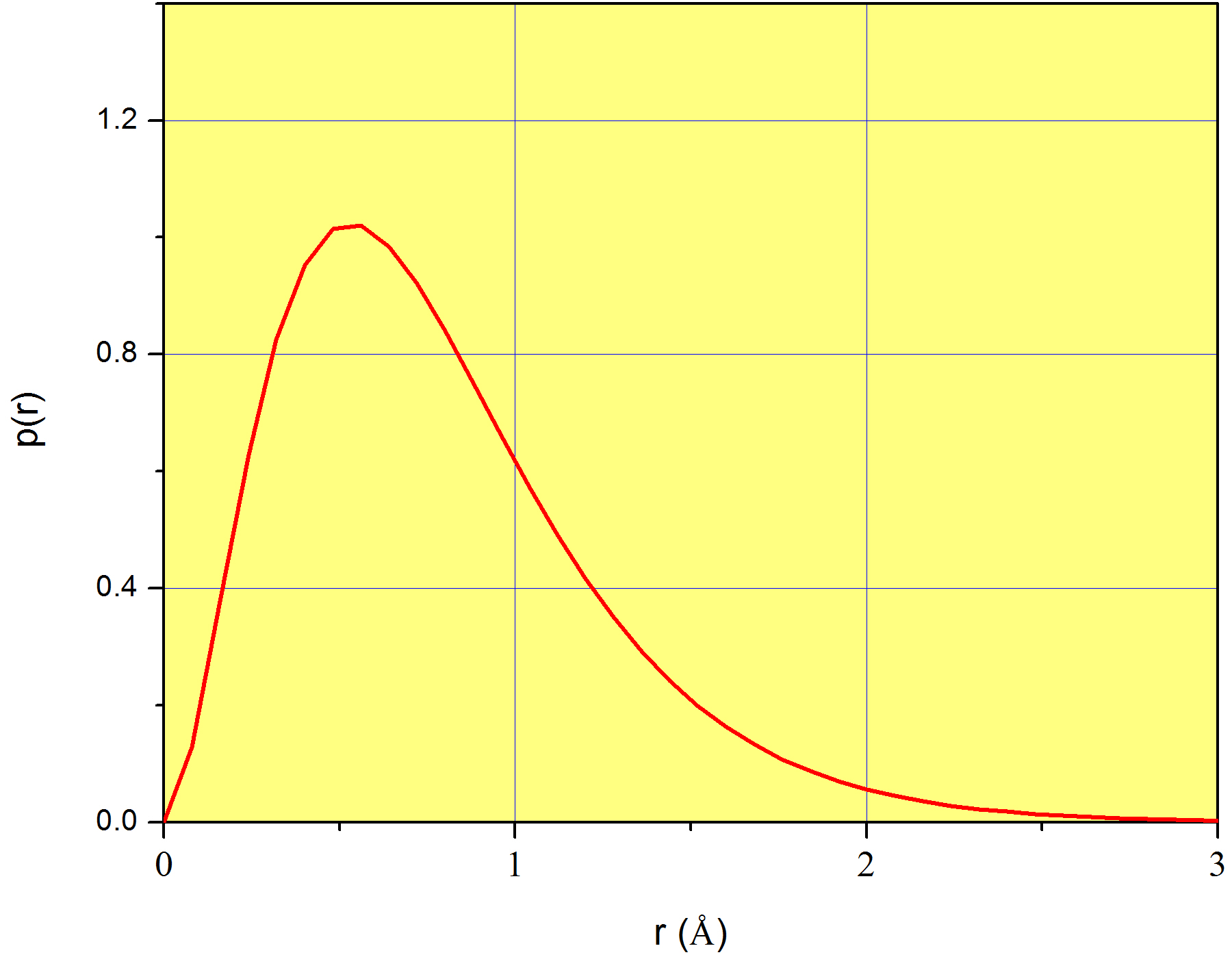
A plot of \(p(r)\) is shown in Figure \(\PageIndex{1}\) for the case of the 1s orbital of the hydrogen atom. Again, we stress that \(p(r)\) does not measure the probability corresponding to each value of \(r\) (which is zero for all values of \(r\)), but instead, it measures a probability density. We already introduced this idea in page
Formally, the probability density function (\(p(r)\)), is defined in this way:
\[\label{eq:coordinates_pdf} P(a\leq r\leq b)=\int\limits_{a}^{b}p(r)dr\]
This means that the probability that the random variable \(r\) takes a value in the interval \([a,b]\) is the integral of the probability density function from \(a\) to \(b\). For a very small interval:
\[\label{eq:coordinates_pdf2} P(a\leq r\leq a+dr)=p(a)dr\]
In conclusion, although \(p(r)\) alone does not mean anything physically, \(p(r)dr\) is the probability that the variable \(r\) takes a value in the interval between \(r\) and \(r+dr\). For example, coming back to Figure \(\PageIndex{1}\), \(p(1\) Å) = 0.62, which does not mean at all that 62% of the time we’ll find the electron at exactly 1Å from the nucleus. Instead, we can use it to calculate the probability that the electron is found in a very narrow region around 1Å . For example, \(P(1\leq r\leq 1.001)\approx 0.62\times 0.001=6.2\times 10^{-4}\). This is only an approximation because the number 0.001, although much smaller than 1, is not an infinitesimal.
In general, the concept of probability density function is easier to understand in the context of Equation \ref{eq:coordinates_pdf}. You can calculate the probability that the electron is found at a distance shorter than 1Å as:
\[P(0\leq r\leq 1)=\int\limits_{0}^{1}p(r)dr \nonumber\]
and at a distance larger than 1Å but shorter than 2Å as
\[P(1\leq r\leq 2)=\int\limits_{1}^{2}p(r)dr \nonumber\]
Of course the probability that the electron is somewhere in the universe is 1, so:
\[P(0\leq r\leq \infty)=\int\limits_{0}^{\infty}p(r)dr=1 \nonumber\]
We haven’t written \(p(r)\) explicitly yet, but we will do so shortly so we can perform all these integrations and get the probabilities discussed above.
Confused about continuous probability density functions? This video may help! http: //tinyurl.com/m6tgoap
The Mean of a Continuous Distribution
For a continuous random variable \(x\), Equation \ref{eq:mean_discrete} becomes:
\[\label{eq:mean_continuous} \left \langle x \right \rangle = \int\limits_{all\,outcomes}p(x) x \;dx\]
Coming back to our atom:
\[\label{eq:mean_r} \left \langle r \right \rangle = \int\limits_{0}^{\infty}p(r) r \;dr\]
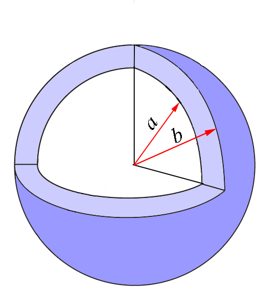
Again, we will come back to this equation once we obtain the expression for \(p(r)\) we need. But before doing so, let’s expand this discussion to more variables. So far, we have limited our discussion to one coordinate, so the quantity \(P(a\leq r\leq b)=\int\limits_{a}^{b}p(r)dr\) represents the probability that the coordinate \(r\) takes a value between \(a\) and \(b\), independently of the values of \(\theta\) and \(\phi\). This region of space is the spherical shell represented in Figure \(\PageIndex{2}\) in light blue. The spheres in the figure are cut for clarity, but of course we refer to the whole shell that is defined as the region between two concentric spheres of radii \(a\) and \(b\).
What if we are interested in the angles as well? Let’s say that we want the probability that the electron is found between \(r_1\) and \(r_2\), \(\theta_1\) and \(\theta_2\), and \(\phi_1\) and \(\phi_2\). This volume is shown in Figure \(\PageIndex{3}\). The probability we are interested in is:
\[P(r_1\leq r\leq r_2, \theta_1\leq \theta \leq \theta_2, \phi_1 \leq \phi \leq\phi_2)=\int\limits_{\phi_1}^{\phi_2}\int\limits_{\theta_1}^{\theta_2}\int\limits_{r_1}^{r_2}p(r,\theta,\phi)\;r^2 \sin\theta dr d\theta d\phi \nonumber\]
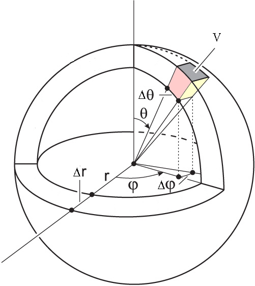
Notice that we are integrating in spherical coordinates, so we need to use the corresponding differential of volume.
This probability density function, \(p(r,\theta,\phi)\), is exactly what \(|\psi(r,\theta,\phi)|^2\) represents! This is why we’ve been saying that \(|\psi(r,\theta,\phi)|^2\) is a probability density. The function \(|\psi(r,\theta,\phi)|^2\) does not represent a probability in itself, but it does when integrated between the limits of interest. Suppose we want to know the probability that the electron in the 1s orbital of the hydrogen atom is found between \(r_1\) and \(r_2\), \(\theta_1\) and \(\theta_2\), and \(\phi_1\) and \(\phi_2\). The answer to this question is:
\[\int\limits_{\phi_1}^{\phi_2}\int\limits_{\theta_1}^{\theta_2}\int\limits_{r_1}^{r_2}|\psi_{1s}|^2\;r^2 \sin\theta dr d\theta d\phi \nonumber\]
Coming back to the case shown in Figure \(\PageIndex{2}\), the probability that \(r\) takes a value between \(a\) and \(b\) independently of the values of the angles, is the probability that \(r\) lies between \(a\) and \(b\), and \(\theta\) takes a value between 0 and \(\pi\), and \(\phi\) takes a value between 0 and \(2\pi\):
\[\label{eq:coordinates9} P(a\leq r\leq b)=P(a\leq r\leq b,0 \leq \theta \leq \pi, 0 \leq \phi \leq 2\pi)=\int\limits_{0}^{2\pi}\int\limits_{0}^{\pi}\int\limits_{a}^{b}|\psi_{1s}|^2\;r^2 \sin\theta dr d\theta d\phi\]
The Radial Density Function
So far we established that \(|\psi(r,\theta,\phi)|^2\) is a probability density function in spherical coordinates. We can perform triple integrals to calculate the probability of finding the electron in different regions of space (but not in a particular point!). It is often useful to know the likelihood of finding the electron in an orbital at any given distance away from the nucleus. This enables us to say at what distance from the nucleus the electron is most likely to be found, and also how tightly or loosely the electron is bound in a particular atom. This is expressed by the radial distribution function, \(p(r)\), which is plotted in Figure \(\PageIndex{1}\) for the 1s orbital of the hydrogen atom.
In other words, we want a version of \(|\psi(r,\theta,\phi)|^2\) that is independent of the angles. This new function will be a function of \(r\) only, and can be used, among other things, to calculate the mean of \(r\), the most probable value of \(r\), the probability that \(r\) lies in a given range of distances, etc.
We already introduced this function in Equation \ref{eq:coordinates_pdf}. The question now is, how do we obtain \(p(r)\) from \(|\psi(r,\theta,\phi)|^2\)? Let’s compare Equation \ref{eq:coordinates_pdf} with Equation \ref{eq:coordinates9}:
\[P(a\leq r\leq b)=\int\limits_{a}^{b}p(r)dr \nonumber\]
\[P(a\leq r\leq b)=P(a\leq r\leq b,0 \leq \theta \leq \pi, 0 \leq \phi \leq 2\pi)=\int\limits_{0}^{2\pi}\int\limits_{0}^{\pi}\int\limits_{a}^{b}|\psi(r,\theta,\phi)|^2\;r^2 \sin\theta dr d\theta d\phi \nonumber\]
We conclude that
\[\int\limits_{a}^{b}p(r)dr=\int\limits_{0}^{2\pi}\int\limits_{0}^{\pi}\int\limits_{a}^{b}|\psi(r,\theta,\phi)|^2\;r^2 \sin\theta dr d\theta d\phi \nonumber\]
All \(s\) orbitals are real functions of \(r\) only, so \(|\psi(r,\theta,\phi)|^2\) does not depend on \(\theta\) or \(\phi\). In this case:
\[\int\limits_{a}^{b}p(r)dr=\int\limits_{0}^{2\pi}\int\limits_{0}^{\pi}\int\limits_{a}^{b}\psi^2(r)\;r^2 \sin\theta dr d\theta d\phi=\int\limits_{0}^{2\pi}d\phi \int\limits_{0}^{\pi}\sin\theta \;d\theta \int\limits_{a}^{b}\psi^2(r)\;r^2 dr=4\pi\int\limits_{a}^{b}\psi^2(r)\;r^2 dr \nonumber\]
Therefore, for an \(s\) orbital,
\[p(r)=4\pi\psi^2(r)\;r^2 \nonumber\]
For example, the normalized wavefunction of the 1s orbital is the solution of Example \(10.1\): \(\dfrac{1}{\sqrt{\pi a_0^3}}e^{-r/a_0}\). Therefore, for the 1s orbital:
\[\label{eq:coordinates10} p(r)=\dfrac{4}{a_0^3}r^2e^{-2r/a_0}\]
Equation \ref{eq:coordinates10} is plotted in Figure \(\PageIndex{1}\). In order to create this plot, we need the value of \(a_0\), which is a constant known as Bohr radius, and equals \(5.29\times10^{-11}m\) (or 0.526 Å). Look at the position of the maximum of \(p(r)\); it is slightly above 0.5Å and more precisely, exactly at \(r=a_0\)! Now it is clear why \(a_0\) is known as a radius: it is the distance from the nucleus at which finding the only electron of the hydrogen atom is greatest. In a way, \(a_0\) is the radius of the atom, although we know this is not strictly true because the electron is not orbiting at a fixed \(r\) as scientists believed a long time ago.
In general, for any type of orbital,
\[\int\limits_{a}^{b}p(r)dr=\int\limits_{0}^{2\pi}\int\limits_{0}^{\pi}\int\limits_{a}^{b}|\psi(r,\theta,\phi)|^2\;r^2 \sin\theta dr d\theta d\phi=\int\limits_{a}^{b}{\color{Red}\int\limits_{0}^{2\pi}\int\limits_{0}^{\pi}|\psi(r,\theta,\phi)|^2\;r^2 \sin\theta\; d\theta d\phi} dr \nonumber\]
in the right side of the equation, we just changed the order of integration to have \(dr\) last, and color coded the expression so we can easily identify \(p(r)\) as:
\[\label{eq:p(r)} p(r)=\int\limits_{0}^{2\pi}\int\limits_{0}^{\pi}|\psi(r,\theta,\phi)|^2\;r^2 \sin\theta\; d\theta d\phi\]
Equation \ref{eq:p(r)} is the mathematical formulation of what we wanted: a probability density function that does not depend on the angles. We integrate \(\phi\) and \(\theta\) so what we are left with represents the dependence with \(r\).
We can multiply both sides by \(r\):
\[rp(r)=r\int\limits_{0}^{2\pi}\int\limits_{0}^{\pi}{\color{Red}|\psi(r,\theta,\phi)|^2}{\color{OliveGreen}r^2 \sin\theta\; d\theta d\phi}=\int\limits_{0}^{2\pi}\int\limits_{0}^{\pi}{\color{Red}|\psi(r,\theta,\phi)|^2}r{\color{OliveGreen}r^2 \sin\theta\; d\theta d\phi} \nonumber\]
and use Equation \ref{eq:mean_r} to calculate \(\left \langle r \right \rangle\)
\[\label{eq:coordinates12} \left \langle r \right \rangle = \int\limits_{0}^{\infty}{\color{Magenta}p(r) r} \;dr=\int\limits_{0}^{\infty}{\color{Magenta}\int\limits_{0}^{2\pi}\int\limits_{0}^{\pi}|\psi(r,\theta,\phi)|^2r\;r^2 \sin\theta\; d\theta d\phi}dr\]
The colors in these expressions are aimed to help you track where the different terms come from.
Let’s look at Equation \ref{eq:coordinates12} more closely. Basically, we just concluded that:
\[\label{eq:coordinates13} \left \langle r \right \rangle = \int\limits_{all\;space}|\psi|^2r\;dV\]
where \(dV\) is the differential of volume in spherical coordinates. We know that \(\psi\) is normalized, so
\[\int\limits_{all\;space}|\psi|^2\;dV=1 \nonumber\]
If we multiply the integrand by \(r\), we get \(\left \langle r \right \rangle\). We will discuss an extension of this idea when we talk about operators. For now, let’s use Equation \ref{eq:coordinates13} to calculate \(\left \langle r \right \rangle\) for the 1s orbital.
Calculate the average value of \(r\), \(\left \langle r \right \rangle\), for an electron in the 1s orbital of the hydrogen atom. The normalized wavefunction of the 1s orbital, expressed in spherical coordinates, is:
\[\psi_{1s}=\dfrac{1}{\sqrt{\pi a_0^3}}e^{-r/a_0} \nonumber\]
Solution
The average value of \(r\) is:
\[\left \langle r \right \rangle=\int\limits_{0}^{\infty}p(r)r\;dr \nonumber\]
or
\[\left \langle r \right \rangle = \int\limits_{all\;space}|\psi|^2r\;dV \nonumber\]
The difference between the first expression and the second expression is that in the first case, we already integrated over the angles \(\theta\) and \(\phi\). The second expression is a triple integral because \(|\psi|^2\) still retains the angular information.
We do not have \(p(r)\), so either we obtain it first from \(|\psi|^2\), or directly use \(|\psi|^2\) and perform the triple integration:
\[\left \langle r \right \rangle = \int\limits_{0}^{\infty}\int\limits_{0}^{2\pi}\int\limits_{0}^{\pi}|\psi(r,\theta,\phi)|^2r\;{\color{Red}r^2 \sin\theta\; d\theta d\phi dr} \nonumber\]
The expression highlighted in red is the differential of volume.
For this orbital,
\[|\psi(r,\theta,\phi)|^2=\dfrac{1}{\pi a_0^3}e^{-2r/a_0} \nonumber\]
and then,
\[\left \langle r \right \rangle = \dfrac{1}{\pi a_0^3}\int\limits_{0}^{\infty}e^{-2r/a_0}r^3\;dr\int\limits_{0}^{2\pi}d\phi\int\limits_{0}^{\pi}\sin\theta\; d\theta=\dfrac{4}{a_0^3}\int\limits_{0}^{\infty}e^{-2r/a_0}r^3\;dr \nonumber\]
From the formula sheet:
\(\int_{0}^{\infty}x^ne^{-ax}dx=\dfrac{n!}{a^{n+1}},\; a>0, n\) is a positive integer.
Here, \(n=3\) and \(a= 2/a_0\).
\[\dfrac{4}{a_0^3}\int\limits_{0}^{\infty}r^3e^{-2r/a_0}\;dr=\dfrac{4}{a_0^3}\times \dfrac{3!}{(2/a_0)^4}=\dfrac{3}{2}a_0 \nonumber\]
\[\displaystyle{\color{Maroon}\left \langle r \right \rangle=\dfrac{3}{2}a_0} \nonumber\]
From Example \(\PageIndex{1}\), we notice that on average we expect to see the electron at a distance from the nucleus equal to 1.5 times \(a_0\). This means that if you could measure \(r\), and you perform this measurement on a large number of atoms of hydrogen, or on the same atom many times, you would, on average, see the electron at a distance from the nucleus \(r=1.5 a_0\). However, the probability of seeing the electron is greatest at \(r=a_0\) (page ). We see that the average of a distribution does not necessarily need to equal the value at which the probability is highest2.