7.1: Introduction to Fourier Series
- Page ID
- 106841

In Chapter 3 we learned that a function \(f(x)\) can be expressed as a series in powers of \(x\) as long as \(f(x)\) and all its derivatives are finite at \(x=0\). We then extended this idea to powers of \(x-h\), and called these series “Taylor series”. If \(h=0\), the functions that form the basis set are the powers of \(x: x^0, x^1, x^2...\), and in the more general case of \(h\neq0\), the basis functions are \((x-h)^0, (x-h)^1, (x-h)^2...\)
The powers of \(x\) or \((x-h)\) are not the only choice of basis functions to expand a function in terms of a series. In fact, if we want to produce a series which will converge rapidly, so that we can truncate if after only a few terms, it is a good idea to choose basis functions that have as much as possible in common with the function to be represented. If we want to represent a periodic function, it is useful to use a basis set containing functions that are periodic themselves. For example, consider the following set of functions: \(\sin{(nx)},\;n=1, 2, ..., \infty\):
We can mix a finite number of these functions to produce a periodic function like the one shown in the left panel of Figure \(\PageIndex{2}\), or an infinite number of functions to produce a periodic function like the one shown on the right. Notice that an infinite number of sine functions creates a function with straight lines! We will see that we can create all kinds of periodic functions by just changing the coefficients (i.e. the numbers multiplying each sine function).
So far everything sounds fine, but we have a problem. The functions \(\sin{nx}\) are all odd, and therefore any linear combination will produce an odd periodic function. We might need to represent an even function, or a function that is neither odd nor even. This tells us that we need to expand our basis set to include even functions, and I hope you will agree the obvious choice are the cosine functions \(\cos{(nx)}\).
Below are two examples of even periodic functions that are produced by mixing a finite (left) or infinite (right) number of cosine functions. Notice that both are even functions.
Before moving on, we need to review a few concepts. First, since we will be dealing with periodic functions, we need to define the period of a function. As we saw in Section 1.4, a function \(f(x)\) is said to be periodic with period \(P\) if \(f(x)=f(x+P)\). For example, the period of the function of Figure \(\PageIndex{4}\) is \(2\pi\).
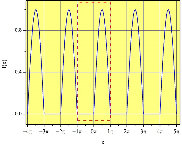
How do we write the equation for this periodic function? We just need to specify the equation of the function between \(-P/2\) and \(P/2\). This range is shown in a red dotted line in Figure \(\PageIndex{4}\), and as you can see, it has the width of a period, and it is centered around \(x=0\). If we have this information, we just need to extend the function to the left and to the right to create the periodic function: