
5.4: An example in Quantum Mechanics
- Page ID
- 106830

The main postulate of quantum mechanics establishes that the state of a quantum mechanical system is specified by a function called the wave function. The wave function is a function of the coordinates of the particle (the position) and time. We often deal with stationary states, i.e. states whose energy does not depend on time. For example, at room temperature and in the absence of electromagnetic radiation such as UV light, the energy of the only electron in the hydrogen atom is constant (the energy of the 1s orbital). In this case, all the information about the state of the particle is contained in a time-independent function, \(\psi (\textbf{r})\), where \(\textbf{r}\) is a vector that defines the position of the particle. In Section 2.3 we briefly mentioned that \(|\psi|^2 = \psi^* \psi\) can be interpreted in terms of the probability of finding the electron in different regions of space. Because the probability of finding the particle somewhere in the universe is 1, the wave function needs to be normalized (that is, the integral of \(|\psi|^2\) over all space has to equal 1).
The fundamental equation in quantum mechanics is known as the Schrödinger equation, which is a differential equation whose solutions are the wave functions. For a particle of mass \(m\) moving in one dimension in a potential field described by \(U(x)\) the Schrödinger equation is:
\[ -\frac{\hbar^2}{2m} \frac{d^2\psi(x)}{dx^2}+U(x)\psi(x)=E \psi(x)\]
Notice that the position of the particle is defined by \(x\), because we are assuming one-dimensional movement. The constant \(\hbar\) (pronounced “h-bar”) is defined as \(h/(2\pi)\), where \(h\) is Plank’s constant. \(U(x)\) is the potential energy the particle is subjected to, and depends on the forces involved in the system. For example, if we were analyzing the hydrogen atom, the potential energy would be due to the force of interaction between the proton (positively charged) and the electron (negatively charged), which depends on their distance. The constant \(E\) is the total energy, equal to the sum of the potential and kinetic energies.
This will be confusing until we start seeing a few examples, so don’t get discouraged and be patient. Let’s start by discussing the simplest (from the mathematical point of view) quantum mechanical system. Our system consists of a particle of mass \(m\) that can move freely in one dimension between two “walls”. The walls are impenetrable, and therefore the probability that you find the particle outside this one-dimensional box is zero. This is not too different from a ping-pong ball bouncing inside a room. It does not matter how hard you bounce the ball against the wall, you will never find it on the other side. However, we will see that for microscopic particles (small mass), the system behaves very different than for macroscopic particles (the ping-pong ball). The behavior of macroscopic systems is described by the laws of what we call classical mechanics, while the behavior of molecules, atoms and sub-atomic particles is described by the laws of quantum mechanics. The problem we just described is known as the “particle in the box” problem, and can be extended to more dimensions (e.g. the particle can move in a 3D box) or geometries (e.g. the particle can move on the surface of a sphere, or inside the area of a circle).
The particle in a one-dimensional box
We will start with the simplest case, which is a problem known as ’the particle in a one-dimensional box’ (Figure \(\PageIndex{1}\)). This is a simple physical problem that, as we will see, provides a rudimentary description of conjugated linear molecules. In this problem, the particle is allowed to move freely in one dimension inside a ’box’ of length \(L\). In this context, ’freely’ means that the particle is not subject to any force, so the potential energy inside the box is zero. The particle is not allowed to move outside the box, and physically, we guarantee this is true by impossing an infinite potential energy at the edges of the box (\(x = 0\) and \(x = L\)) and outside the box (\(x < 0\) and \(x > L\)).
\[U(x)=\left\{\begin{matrix} \infty & x<0 \\ 0 & 0<x<L\\ \infty & x>L \end{matrix}\right. \nonumber\]
Because the potential energy outside the box is infinity, the probability of finding the particle in these regions is zero. This means that \(\psi(x)=0\) if \(x>L\) or \(x<0\). What about \(\psi(x)\) inside the box? In order to find the wave functions that describe the states of a system, we have to solve Schrödinger’s equation:
\[-\frac{\hbar^2}{2m} \frac{d^2\psi(x)}{dx^2}+U(x)\psi(x)=E \psi(x) \nonumber\]
Inside the box \(U(x)=0\), so:
\[-\frac{\hbar^2}{2m} \frac{d^2\psi(x)}{dx^2}=E \psi(x) \nonumber\]
\[ \label{eqn1} \frac{\hbar^2}{2m} \frac{d^2\psi(x)}{dx^2}+ E\psi(x)=0\]
Remember that \(\hbar\) is a constant, \(m\) is the mass of the particle (also constant), and \(E\) the energy. The energy of the particle is a constant in the sense that it is not a function of \(x\). We will see that there are many (in fact infinite) possible values for the energy of the particle, but these are numbers, not functions of \(x\). With all this in mind, hopefully you will recognize that the Schrödinger equation for the one-dimensional particle in a box is a homogeneous second order ODE with constant coefficients. Do we have any initial or boundary conditions? In fact we do, because the wave function needs to be a continuous function of \(x\). This means that there cannot be sudden jumps of probability density when moving though space. In particular in this case, it means that \(\psi(0)=\psi(L)=0\), because the probability of finding the particle outside the box is zero.
Let’s solve Equation \ref{eqn1}. We need to find the functions \(\psi(x)\) that satisfy the ODE. The auxiliary equation is (remember that \(m, \hbar, E\) are positive constants):
\[\frac{\hbar^2}{2m}\alpha^2+E=0 \nonumber\]
\[\alpha=\pm i \sqrt{\frac{2mE}{\hbar^2}} \nonumber\]
and the general solution is therefore:
\[\psi(x)=c_1e^{i \sqrt{\frac{2mE}{\hbar^2}}x}+c_2e^{-i \sqrt{\frac{2mE}{\hbar^2}}x} \nonumber\]
Because \(\psi(0)=0\):
\[\psi(x)=c_1+c_2=0\rightarrow c_1=-c_2 \nonumber\]
\[\psi(x)=c_1\left(e^{i \sqrt{\frac{2mE}{\hbar^2}}x}-e^{-i \sqrt{\frac{2mE}{\hbar^2}}x}\right) \nonumber\]
This can be simplified using Euler’s relationships: \(e^{ix}-e^{-ix}=2i\sin{x}\)
\[\psi(x)=c_1(2i)\sin{\left(\sqrt{\frac{2mE}{\hbar^2}}x\right)} \nonumber\]
\[\psi(x)=A\sin{\left(\sqrt{\frac{2mE}{\hbar^2}}x\right)} \nonumber\]
In the last step we recognized that \(2ic_1\) is a constant, and called it \(A\).
The second boundary condition is \(\psi(L)=0\):
\[\psi(L)=A\sin{\left(\sqrt{\frac{2mE}{\hbar^2}}L\right)}=0 \nonumber\]
We can make \(A=0\), but this will result in the wave function being zero at all values of \(x\). This is what we called the ‘trivial solution’ before, and although it is a solution from the mathematical point of view, it is not when we think about the physics of the problem. If \(\psi(x)=0\) the probability of finding the particle inside the box is zero. However, the problem states that the particle cannot be found outside, so it has to be found inside with a probability of 1. This means that \(\psi(x)=0\) is not a physically acceptable solution inside the box, and we are forced to consider the situations where
\[\sin{\left(\sqrt{\frac{2mE}{\hbar^2}}L\right)}=0 \nonumber\]
We know the function \(\sin{x}\) is zero at values of \(x\) that are zero, or multiples of \(\pi\):
\[\left(\sqrt{\frac{2mE}{\hbar^2}}L\right)=\pi,2\pi, 3\pi...=n\pi\;(n=1,2,3..\infty) \nonumber\]
This means that our solution is:
\[\psi(x)=A\sin{\left(\frac{n\pi}{L}x\right)} \; (n=1,2,3...\infty) \nonumber\]
Notice that we didn’t consider \(n=0\) because that would again cause \(\psi(x)\) to vanish inside the box. The functions \(\psi(x)\) contain information about the state of the system, and are called the eigenfunctions. What about the energies?
\[\left(\sqrt{\frac{2mE}{\hbar^2}}L\right)=n\pi\rightarrow E=\left(\frac{n\pi}{L}\right)^2\frac{\hbar^2}{2m}\;(n=1, 2, 3...\infty) \nonumber\]
The energies are the eigenvalues of this equation. Notice that there are infinite eigenfunctions, and each one has a defined eigenvalue.
| \(n\) | \(\psi(x)\) | \(E\) |
|---|---|---|
| 1 | \(A\sin{\left(\frac{\pi}{L}x\right)}\) | \(\left(\frac{\pi}{L}\right)^2\frac{\hbar^2}{2m}\) |
| 2 | \(A\sin{\left(\frac{2\pi}{L}x\right)}\) | \(\left(\frac{2\pi}{L}\right)^2\frac{\hbar^2}{2m}\) |
| 3 | \(A\sin{\left(\frac{3\pi}{L}x\right)}\) | \(\left(\frac{3\pi}{L}\right)^2\frac{\hbar^2}{2m}\) |
The lowest energy state is described by the wave function \(\psi=A\sin{\left(\frac{\pi}{L}x\right)}\), and its energy is \(\left(\frac{\pi}{L}\right)^2\frac{\hbar^2}{2m}\).
What about the constant \(A\)? Mathematically, any value would work, and none of the boundary conditions impose any restriction on its value. Physically, however, we have another restriction we haven’t fulfilled yet: the wave function needs to be normalized. The integral of \(|\psi|^2\) over all space needs to be 1 because this function represents a probability.
\[\int_{-\infty}^{\infty}|\psi(x)|^2dx=1 \nonumber\]
However, \(\psi(x)=0\) outside the box, so the ranges \(x<0\) and \(x>L\) do not contribute to the integral. Therefore:
\[\int_{0}^{L}|\psi(x)|^2dx=\int_{0}^{L}A^2\sin^2{\left(\frac{n\pi}{L}x\right)}dx=1 \nonumber\]
We will calculate \(A\) from this normalization condition. Using the primitives found in the formula sheet, we get:
\[\int_{0}^{L}\sin^2{\left(\frac{n\pi}{L}x\right)}dx=L/2 \nonumber\]
and therefore
\[A=\sqrt{\frac{2}{L}} \nonumber\]
We can now write down our normalized wave function as:
\[ \psi(x)=\sqrt{\frac{2}{L}}\sin{\left(\frac{n\pi}{L}x\right)} \; (n=1,2,3...\infty) \]
We solved our first problem in quantum mechanics! Let’s discuss what we got, and what it means. First, because the potential energy inside the box is zero, the total energy equals the kinetic energy of the particle (i.e. the energy due to the fact that the particle is moving from left to right or from right to left). A ping-pong ball inside a macroscopic box can move at any speed we want, so its kinetic energy is not quantized. However, if the particle is an electron, its kinetic energy inside the box can adopt only quantized values of energy: \(E=\left(\frac{n\pi}{L}\right)^2\frac{\hbar^2}{2m}\;(n=1, 2, 3...\infty)\). Interestingly, the particle cannot have zero energy (\(n=0\) is not an option), so it cannot be at rest (our ping-pong ball can have zero kinetic energy without violating any physical law). If a ping-pong ball moves freely inside the box we can find it with equal probability close to the edges or close to the center. Not for an electron in a one-dimensional box! The function \(|\psi(x)|^2\) for the lowest energy state (\(n=1\)) is plotted in Figure \(\PageIndex{2}\). The probability of finding the electron is greater at the center than it is at the edges; nothing like what we expect for a macroscopic system. The plot is symmetric around the center of the box, meaning the probability of finding the particle in the left side is the same as finding it in the right side. That is good news, because the problem is truly symmetric, and there are no extra forces attracting or repelling the particle on the left or right half to the box.
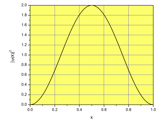
Looking at Figure \(\PageIndex{2}\), you may think that the probability of finding the particle at the center really 2. How can this be? Probabilities cannot be greater than 1! This is a major source of confusion among students, so let’s clarify what it means. The function \(|\psi(x)|^2\) is not a probability, but a probability density. Technically, this means that \(|\psi(x)|^2dx\) is the probability of finding the particle between \(x\) and \(x+dx\) (see page for more details). For example, the probability of finding the particle between \(x=0.5\) and \(0.5001\) is \(\approx|\psi(0.5)|^2\times 0.0001= 0.0002\). This is approximate because \(\Delta x= 0.0001\) is small, but not infinitesimal. What about the probability of finding the particle between \(x=0.5\) and \(0.6\)? We need to integrate \(|\psi(x)|^2dx\) between \(x=0.5\) and \(x=0.6\):
\[p(0.5<x<0.6)=\int_{0.5}^{0.6} |\psi(x)|^2dx\approx 0.2 \nonumber\]
Importantly,
\[p(0<x<1)=\int_{0}^{1} |\psi(x)|^2dx=1 \nonumber\]
as it should be the case for a normalized wave function. Notice that these probabilities refer to the lowest energy state (\(n=1\)), and will be different for states of increasing energy.
The particle in the box problem is also available in video format: http://tinyurl.com/mjsmd2a
Where is the chemistry?
So far we talked about a system that sounds pretty far removed from anything we (chemists) care about. We understand electrons in atoms, but electrons moving in a one-dimensional box? To see why this is not such a crazy idea, let’s consider the molecule of carotene (the orange pigment in carrots). We know that all those double bonds are conjugated, meaning that the \(\pi\) electrons are delocalized and relatively free to move around the bonds highlighted in red in Figure \(\PageIndex{3}\).
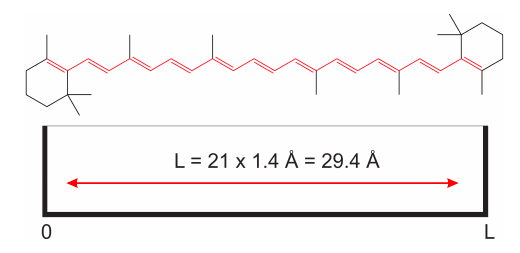
Because the length of each carbon-carbon bond is around 1.4 Å (Å stands for angstrom, and equals \(10^{-10}m\)), we can assume that the \(\pi\) electrons move inside a one dimensional box of length \(L = 21\times 1.4\) Å\(= 29.4\) Å. This is obviously an approximation, as it is not true that the electrons move freely without being subject to any force. Yet, we will see that this simple model gives a good semi-quantitative description of the system.
We already solved the problem of the particle in a box, and obtained the following eigenvalues:
\[ E=\left(\frac{n\pi}{L}\right)^2\frac{\hbar^2}{2m}\;(n=1, 2, 3...\infty) \label{eqn2}\]
These are the energies that the particle in the box is allowed to have. In this case, the particle in question is an electron, so \(m\) is the mass of an electron. Notice that we have everything we need to use Equation \ref{eqn2}: \(\hbar = 1.0545 \times 10^{-34} m^2 kg\, s^{-1}\), \(m=9.109 \times 10^{-31}kg\), and \(L = 2.94 \times 10^{-9} m\). This will allow us to calculate the allowed energies for the \(\pi\) electrons in carotene. For \(n=1\) (the lowest energy state), we have:
\[E_1=\left(\frac{\pi}{L}\right)^2\frac{\hbar^2}{2m}=6.97 \times 10^{-21}J \nonumber\]
Joule is the unit of energy, and \(1J = kg\times m^2\times s^{-2}\). A very easy way of remembering this is to recall Einstein’s equation: \(E = mc^2\), which tells you that energy is a mass times the square of a velocity (hence, \(1J = 1kg (1 m/s)^2\)). Coming back to Equation \ref{eqn2}, the allowed energies for the \(\pi\) electrons in carotene are:
\[E_n=n^2\times6.97 \times 10^{-21}J\;(n=1, 2, 3...\infty) \nonumber\]
Notice that the energies increase rapidly. The energy of the tenth level (\(E_{10}\)) is one hundred times the energy of the first! The number of levels is inifinite, but of course we know that the electrons will fill the ones that are lower in energy. This is analogous to the hydrogen atom. We know there are an infinite number of energy levels, but in the absence of an external energy source we know the electron will be in the 1s orbital, which is the lowest energy level. This electron has an infinite number of levels available, but we need an external source of energy if we want the electron to occupy a higher energy state. The same concepts apply to molecules. As you have learned in general chemistry, we cannot have more than two electrons in a given level, so we will put our 22 \(\pi\) electrons (2 per double bond) in the first 11 levels (Figure \(\PageIndex{4}\), left).
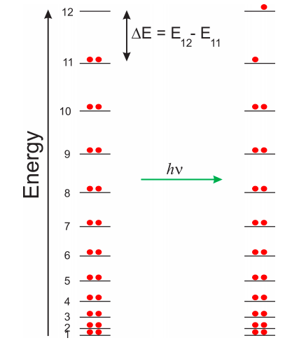
We can promote an electron to the first unoccupied level (in this case \(n=12\)) by using light of the appropriate frequency (\(\nu\)). The energy of a photon is \(E = h\nu\), where \(h\) is Plank’s constant. In order for the molecule to absorb light, the wavelength of the light beam needs to match exactly the gap in energy between the highest occupied state (in this case \(n=11\)) and the lowest unoccupied state. The wavelength of light is related to the frequency as: \(\lambda = c/\nu\), where \(c\) is the speed of light. Therefore, in order to produce the excited state shown in the right side of Figure \(\PageIndex{4}\), we have to use light of the following wavelength:
\[E=E_{12}-E_{11}=h\nu=h c/\lambda\rightarrow \lambda=hc/(E_{12}-E_{11}) \nonumber\]
Recall that \(E_n=n^2\times6.97 \times 10^{-21}J\), so \((E_{12}-E_{11})= (144-121)\times6.97 \times 10^{-21}J=1.60\times 10^{-19}J\). Therefore,
\[\lambda = \frac{6.626\times10^{-34} J\,s\times 3\times10^8 m\, s^{-1}}{1.60\times 10^{-19}J}=1.24\times10^{-6}m=1,242 nm \nonumber\]
In the last step we expressed the result in nanometers (\(1nm=10^{-9}m\)), which is a common unit to describe the wavelength of light in the visible and ultraviolet regions of the electromagnetic spectrum. It is actually fairly easy to measure the absorption spectrum of carotene. You just need to have a solution of carotene, shine the solution with light of different colors (wavelengths), and see what percentage of the light is transmitted. The light that is not transmitted is absorbed by the molecules due to transitions such as the one shown in Figure \(\PageIndex{4}\). In reality, the absorption of carotene actually occurs at 497 nm, not at 1,242 nm. The discrepancy is due to the huge approximations of the particle in the box model. Electrons are subject to interactions with other electrons, and with the nuclei of the atoms, so it is not true that the potential energy is zero. Although the difference seems large, you should not be too disappointed about the result. It is actually pretty impressive that such a simple model can give a prediction that is not that far from the experimental result. Nowadays chemists use computers to analyze more sophisticated models that cannot be solved analytically in the way we just solved the particle in the box. Yet, there are some qualitative aspects of the particle in the box model that are useful despite the approximations. One of these aspects is that the wavelength of the absorbed light gets lower as we reduce the size of the box. From Equation \ref{eqn2}, we can write:
\[h c/\lambda=\left(\frac{\pi}{L}\right)^2\frac{\hbar^2}{2m}(n_2^2-n_1^2) \nonumber\]
where \(n_2\) is the lowest unoccupied level, and \(n_1\) is the highest occupied level. Because \(n_2=n_1+1\),
\[h c/\lambda=\left(\frac{\pi}{L}\right)^2\frac{\hbar^2}{2m}((n_1+1)^2-n_1^2)=\left(\frac{\pi}{L}\right)^2\frac{\hbar^2}{2m}(2n_1+1) \nonumber\]
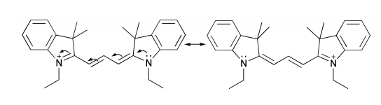
Molecules that have a longer conjugated system will absorb light of longer wavelengths (less energy), and molecules with a shorter conjugated system will absorb light of shorter wavelengths (higher energy). For example, consider the following molecule, which is a member of a family of fluorescent dyes known as cyanines. The conjugated system contains 8 \(\pi\) electrons, and the molecule absorbs light of around 550 nm. This wavelength corresponds to the green region of the visible spectrum. The solution absorbs green and lets everything else reach your eye. Red is the complementary color of green, so this molecule in solution will look red to you.
Now look at this other cyanine, which has two extra \(\pi\) electrons:
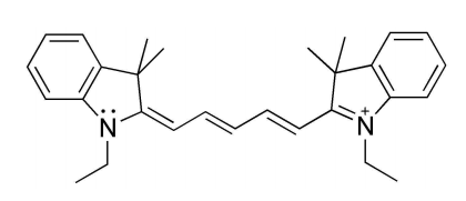
The particle in a box model tells you that this cyanine should absorb light of longer wavelengths (less energy), so it should not surprise you to know that a solution of this compound absorbs light of about 670 nm. This corresponds to the orange-red region of the spectrum, and the solution will look blue to us. If we instead shorten the conjugated chain we will produce a compound that absorbs in the blue (450 nm), and that will be yellow when in solution. We just connected differential equations, quantum mechanics and the colors of things... impressive!