
4.1: Definitions and General Concepts
- Page ID
- 106820

A differential equation is an equation that defines a relationship between a function and one or more derivatives of that function.
For example, this is a differential equation that relates the function \(y(t)\) with its first and second derivatives:
\[\dfrac{d^2}{dt^2}y(t)+\dfrac{1}{4}\dfrac{d}{dt}y(t)+y(t)=\sin(t) \nonumber\]
The above example is an ordinary differential equation (ODE) because the unknown function, \(y(t)\), is a function of a single variable (in this case \(t\)). Because we are dealing with a function of a single variable, only ordinary derivatives appear in the equation. If we were dealing with a function of two or more variables, the partial derivatives of the function would appear in the equation, and we would call this differential equation a partial differential equation (PDE). An example of a PDE is shown below. We will discuss PDEs towards the end of the semester.
\[\dfrac{\partial ^2u}{\partial x^2}+\dfrac{\partial ^2u}{\partial y^2}+\dfrac{\partial ^2u}{\partial z^2}=c^2 \dfrac{\partial ^2u}{\partial t^2} \nonumber\]
Note that in the example above we got ‘lazy’ and used \(u\) instead of \(u(x,y,z,t)\). The fact that \(u\) is a function of \(x,y,z\), and \(t\) is obvious from the derivatives, so you will see that often we will relax and not write the variables explicitly with the function.
Why do we need to study differential equations? The answer is simple: Differential equations arise in the mathematical models that describe most physical processes. Figure \(\PageIndex{1}\) illustrates three examples.
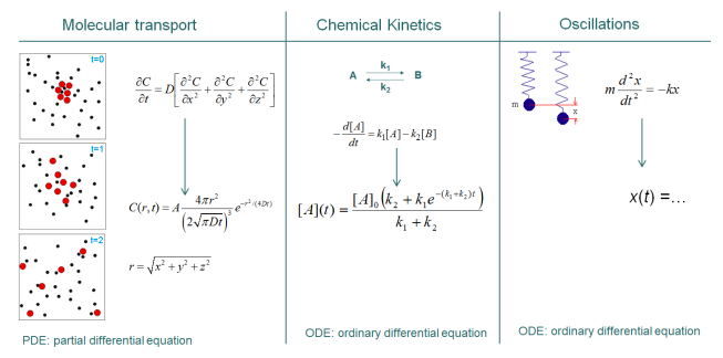
The first column illustrates the problem of molecular transport (diffusion). Suppose the red circles represent molecules of sucrose (sugar) and the black circles molecules of water, and assume you are interested in modeling the concentration of sucrose as a function of position and time after you dissolve some sucrose right in the middle of the container. The differential equation describing the process is a partial differential equation because the concentration will be a function of two variables: \(r\), the distance from the origin, and \(t\), the time elapsed from the moment you started the experiment. The solution shown in the figure was obtained by assuming that all the molecules of sucrose are concentrated at the center at time zero. You could solve the differential equation with other initial conditions.
The second column illustrates a chemical system where a compound A reacts to give B. The reaction is reversible, and it could, for example, represent two different isomers of the same molecule. The differential equation models how the concentration of A, [A], changes with time. We will in fact analyze this problem in detail and find the solution shown in the figure. As we will see, in this case we are also assuming certain initial conditions.
Finally, the third column illustrates a mass attached to a spring. We will also analyze this equation, and the solution is not shown because it will be your job to get it in your homework. You may think this is a physics problem, but because molecules have chemical bonds, and atoms vibrate around their equilibrium positions, systems like these are of interest to chemists as well.
To solve the differential equation means to find the function (or family of functions) that satisfies the equation. In our first example in Figure \(\PageIndex{1}\), we would need to find the function C\((r,t)\) that satisfies the equation. In the second example we would need to find all the functions A\((t)\) that satisfy the equation. As we will see shortly, whether the solution is one function or a family of functions depends on whether we are restricted by initial conditions (e.g. at time zero [B] = 0) or not.
The order of a differential equation (partial or ordinary) is the highest derivative that appears in the equation. Below is an example of a first order ordinary differential equation:
\[\label{eq1}\dfrac{dy}{dx}+3y=8e^x\]
In this example, we are looking for all the functions \(y(x)\) that satisfy Equation \ref{eq1}. As usual, we will call \(x\) the independent variable, and \(y\) the dependent variable. Again, \(y\) is of course \(y(x)\), but often we do not write this explicitly to save space and time. This is an ordinary differential equation because \(y\) is a function of a single variable. It is a first order differential equation because the highest derivative is of first order. It is also a linear differential equation because the dependent variable and all of its derivatives appear in a linear fashion. The distinction between linear and non-linear ODEs is very important because there are different methods to solve different types of differential equations. Mathematically, a first order linear ODE will have this general form:
\[\dfrac{dy}{dx}+f_1(x) y=f_2(x)\]
It is crucial to understand that the linearity refers to the terms that include the dependent variable (in this case \(y\)). The terms involving \(x\) (\(f_1(x)\) and \(f_2(x)\)) can be non-linear, as in Equation \ref{eq1}. An example of a non-linear differential equation is shown below. Note that the dependent variable appears in a transcendental function (in this case an exponential), and that makes this equation non-linear:
\[\dfrac{dy}{dx}+3e^y=8x \nonumber\]
Analogously, a linear second order ODE will have the general form:
\[\label{eq:linear}\dfrac{d^2y}{dx^2}+f_1(x)\dfrac{dy}{dx}+f_2(x) y=f_3(x)\]
Again, we don’t care whether the functions \(f_1(x), f_2(x)\) and \(f_3(x)\) are linear in \(x\) or not. The only thing that matters is that the terms involving the dependent variable are.
Identifying the dependent and the independent variables: Test yourself with this short quiz. http://tinyurl.com/ll22wnv
Linear or non-linear? See if you can identify the linear ODEs in this short quiz. http://tinyurl.com/msldkp3
We are still defining concepts, but we haven’t said anything so far regarding how to solve differential equations! We still need to go over a few more things, so be patient.
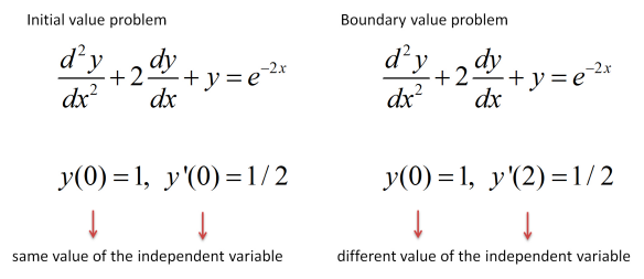
An \(nth\)-order differential equation together with \(n\) auxiliary conditions imposed at the same value of the independent variable is called an initial value problem. For example, we may be interested in finding the function \(y(x)\) that satisfies the following conditions:
\[\label{eq2}y''=e^{-x}, y(0)=1, y'(0)=4\]
Notice that we are introducing different types of notations so you get used to seeing mathematical equations in different ‘flavors’. Here, \(y''\) of course means \(\dfrac{d^2y(x)}{dx^2}\). This is an initial value problem because we have a second-order differential equation with two auxiliary conditions imposed at the same value of \(x\) (in this case \(x=0\)). There are infinite functions \(y(x)\) that satisfy \(y''=e^{-x}\), but only one will also satisfy the two initial conditions we imposed. If we were dealing with a first order differential equation we would need only one initial condition. We would need three for a third-order differential equation.
How do we use initial conditions to find a solution? In general, the solution of a second order ODE will contain two arbitrary constants (in the example below \(c_1\) and \(c_2\)). This is what we will call the general solution of the differential equation. For example,
\(y(x)=e^{-x} + c_1 x+c_2\) is the general solution of \(y''=e^{-x}\). We can verify this is true by taking the second derivative of this function. Again, we do not know yet how to get these solutions, but if we are given this solution, we know how to check if it is correct. It is clear that \(c_1\) and \(c_2\) can be in principle anything, so the solution of the ODE is a whole family of functions. However, if we are given initial conditions we are looking for a particular solution, one that not only satisfies the ODE, but also the initial conditions. Which function is that?
The first initial condition states that \(y(0)=1\). Therefore,
\[y(x)=e^{-x} + c_1 x+c_2\Rightarrow y(0)=1+c_2 \nonumber\]
\[y(0)=1 \Rightarrow 1=1+c_2 \Rightarrow c_2 =0 \nonumber\]
So far, we demonstrated that the functions \(y(x)=e^{-x} + c_1 x\) satisfy not only the ODE, but also the initial condition \(y(0)=1\). We still have another initial condition, which will allow us to determine the value of \(c_1\).
\[y'(x)=-e^{-x} + c_1\Rightarrow y'(0)=-1+c_1 \nonumber\]
\[y'(0)=4 \Rightarrow 4=-1+c_1 \Rightarrow c_1 =5 \nonumber\]
Therefore, the function \(y(x)=e^{-x}+5x\) is the particular solution of the initial value problem described in Equation \ref{eq2}. We can check our answer by verifying that this solution satisfies the three equations of the initial value problem:
- \(y''=e^{-x} \rightarrow\) \(\dfrac{d^2}{dx^2} (e^{-x}+5x)=e^{-x}\), so we know that the solution we found satisfies the differential equation.
- \(y(0)=1 \rightarrow\)e\(^{-0}+5\times 0=1\), so we know that the solution we found satisfies one of the initial conditions.
- \(y'(0)=4 \rightarrow\)\(\dfrac{d}{dx} (e^{-x}+5x)=-e^{-x}+5\Rightarrow y'(0)=4\), so we know that the solution we found satisfies the other initial condition as well.
Therefore, we demonstrated that \(y(x)=e^{-x}+5x\) is indeed the solution of the problem.
An \(nth\)-order differential equation together with \(n\) auxiliary conditions imposed at more than one value of the independent variable is called a boundary value problem. What is the difference between a boundary value problem and an initial value problem? In the first case, the conditions are imposed at different values of the independent variable, while in the second case, as we just saw, the conditions are imposed at the same value of the independent variable. For example, this would be a boundary value problem:
\[\label{eq3}y''=e^{-x}, y(0)=1, y(1)=0\]
Notice that we still have two conditions because we are dealing with a second order differential equation. However, one condition deals with \(x=1\) and the other with \(x=0\). The conditions can refer to values of the first derivative, as in the previous example, or to values of the function itself, as in the example of Equation \ref{eq3}.
Why do we need to distinguish between initial value and boundary value problems? The reason lies in a theorem that states that, for linear ODEs, the solution of a initial value problem exists and is unique, but a boundary value problem does not have the existence and uniqueness guarantee. The theorem is not that simple (for example it requires that the functions in \(x\) (\(f_{1...3}\) in Equation \ref{eq:linear}) are continuous), but the bottom line is that we may find a solution whenever the conditions are imposed at the same value of \(x\), but we may not find a solution whenever the conditions are imposed at different values. We will see examples when we discuss second order ODEs, and in particular we will discuss how boundary conditions give rise to interesting physical phenomena. For example, we will see that boundary conditions are responsible for the fact that energies in atoms and molecules are quantized.
Coming back to the boundary value problem of Equation \ref{eq3}, it is important to recognize that because the actual differential equation is the same as in the example of Equation \ref{eq2}, the general solution is still the same: \(y(x)=e^{-x} + c_1 x+c_2\). However, the particular solution will be different (different values of \(c_1\) and \(c_2\)), because we need to satisfy different conditions.
As in the first example, the first boundary condition states that \(y(0)=1\) so:
\[y(x)=e^{-x} + c_1 x+c_2\Rightarrow y(0)=1+c_2 \nonumber\]
\[y(0)=1 \Rightarrow 1=1+c_2 \Rightarrow c_2 =0 \nonumber\]
as before. However, now
\[y(1)=e^{-1} + c_1 \nonumber\]
where we have used the result \(c_2=0\) so
\[y(1)=0 \Rightarrow 0=e^{-1}+c_1 \Rightarrow c_1 =-e^{-1} \nonumber\]
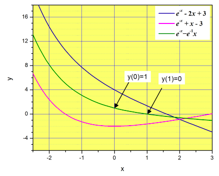
and the particular solution is therefore \(y(x)=e^{-x}-e^{-1}x\). As we did before, it is important that we check our solution. If we are right, this solution needs to satisfy all the relationships stated in Equation \ref{eq3}.
- \(y''=e^{-x} \rightarrow\) \(\dfrac{d^2}{dx^2} (e^{-x}-e^{-1}x)=e^{-x}\), so the solution satisfies the differential equation.
- \(y(0)=1 \rightarrow\)e\(^{-0}-e^{-1}\times 0=1\), so our solution satisfies one of the boundary conditions.
- \(y(1)=0 \rightarrow\)\(e^{-1}-e^{-1}\times1=0\), so our solution satisfies the other boundary condition as well.
Figure \(\PageIndex{3}\) illustrates the difference between the general solution and the particular solution. The general solution has two arbitrary constants, so there are an infinite number of functions that satisfy the differential equation. Three examples are shown in different colors. However, only one of these satisfies both boundary conditions (shown with the arrows).
Using boundary conditions: see if you can obtain the particular solution of a second order ODE in this short quiz. http://tinyurl.com/lovh4x3
So far we have discussed how to:
- Identify the dependent and independent variables
- Identify the order of the differential equation.
- Identify whether the equation is linear or not
- Use initial or boundary conditions to obtain particular solutions from general solutions
- Check your results to be sure you satisfy the differential equation and all the initial or boundary conditions
We are obviously missing the most important question: How do we solve the differential equation? Unfortunately, there is no universal method, and in fact some differential equations cannot be solved analytically. We will see some examples of equations that cannot be solved analytically and we will discuss what can be done in those cases. In this class we will only discuss some differential equations of interest in physical chemistry. It is not our intention to cover the topic in a comprehensive manner, and we will not touch on other differential equations that might be of interest in other disciplines. Yet, the background you will get in this class will allow you to teach yourself more advanced topics in differential equations if your future career demands that you have a deeper knowledge of the subject.