2.9: Vibrations of Molecules

This Schrödinger equation forms the basis for our thinking about bond stretching and angle bending vibrations as well as collective vibrations in solids called phonons.

The radial motion of a diatomic molecule in its lowest (\(J=0\)) rotational level can be described by the following Schrödinger equation:

\[- \dfrac{\hbar^2}{2\mu r^2} \dfrac{\partial}{\partial r} \left(r^2\dfrac{\partial \psi}{\partial r}\right) +V(r) \psi = E \psi,\]

where \(\mu\) is the reduced mass \(\mu = \dfrac{m_1m_2}{m_1+m_2}\) of the two atoms. If the molecule is rotating, then the above Schrödinger equation has an additional term \(J(J+1) \hbar^2/2\mu r^{-2} \psi\) on its left-hand side. Thus, each rotational state (labeled by the rotational quantum number \(J\)) has its own vibrational Schrödinger equation and thus its own set of vibrational energy levels and wave functions. It is common to examine the \(J=0\) vibrational problem and then to use the vibrational levels of this state as approximations to the vibrational levels of states with non-zero \(J\) values (treating the vibration-rotation coupling via perturbation theory). Let us thus focus on the \(J=0\) situation.

By substituting \(\psi= \dfrac{\Phi(r)}{r}\) into this equation, one obtains an equation for \(\Phi(r)\) in which the differential operators appear to be less complicated:

\[- \dfrac{\hbar^2}{2\mu} \dfrac{d^2F}{dr^2} + V(r) \Phi = E F.\]

This equation is exactly the same as the equation seen earlier in this text for the radial motion of the electron in the hydrogen-like atoms except that the reduced mass m replaces the electron mass m and the potential \(V(r)\) is not the Coulomb potential.

If the vibrational potential is approximated as a quadratic function of the bond displacement \(x = r-r_e\) expanded about the equilibrium bond length \(r_e\) where \(V\) has its minimum:

\[V = \dfrac{1}{2} k(r-r_e)^2,\]

the resulting harmonic-oscillator equation can be solved exactly. Because the potential \(V\) grows without bound as \(x\) approaches \(\infty\) or \(-\infty\), only bound-state solutions exist for this model problem. That is, the motion is confined by the nature of the potential, so no continuum states exist in which the two atoms bound together by the potential are dissociated into two separate atoms.

In solving the radial differential equation for this potential, the large-r behavior is first examined. For large-r, the equation reads:

\[\dfrac{d^2F}{dx^2} = \dfrac{1}{2} k x^2 \dfrac{2\mu}{\hbar^2} \Phi = \dfrac{k\mu}{\hbar^2} x^2 F,\]

where \(x = r-r_e\) is the bond displacement away from equilibrium. Defining \(\beta^2 =\dfrac{k\mu}{\hbar^2}\) and \(\xi= \sqrt{\beta} x\) as a new scaled radial coordinate, and realizing that

\[\dfrac{d^2}{dx^2} = \beta \dfrac{d^2}{dx^2}\]

allows the larger Schrödinger equation to be written as:

\[\dfrac{d^2F}{d\xi^2} = \xi^2 F\]

which has the solution

\[F_{\rm large-r} = \exp(- \xi^2/2).\]

The general solution to the radial equation is then expressed as this large-r solution multiplied by a power series in the \(z\) variable:

\[\Phi = \exp(- \xi^2/2)\sum_{n=0}\xi^n C_n ,\]

where the \(C_n\) are coefficients to be determined. Substituting this expression into the full radial equation generates a set of recursion equations for the \(C_n\)​ amplitudes. As in the solution of the hydrogen-like radial equation, the series described by these coefficients is divergent unless the energy \(E\) happens to equal specific values. It is this requirement that the wave function not diverge so it can be normalized that yields energy quantization. The energies of the states that arise by imposing this non-divergence condition are given by:

\[E_n = \hbar \sqrt{\dfrac{k}{\mu}} (n+\dfrac{1}{2}),\]

and the eigenfunctions are given in terms of the so-called Hermite polynomials \(H_n(y)\) as follows:

\[\psi_n(x) = \dfrac{1}{\sqrt{n! 2^n}} \left(\dfrac{\beta}{\pi}\right)^{1/4} \exp(- \beta \xi^2/2) H_n(\sqrt{\beta} x),\]

where \(\beta =\sqrt{\dfrac{k}{\mu}}\). Within this harmonic approximation to the potential, the vibrational energy levels are evenly spaced:

\[\Delta E = E_{n+1} - E_n = \hbar \sqrt{\dfrac{k}{\mu}} .\]

In experimental data such evenly spaced energy level patterns are seldom seen; most commonly, one finds spacings \(E_{n+1} - E_n\) that decrease as the quantum number \(n\) increases. In such cases, one says that the progression of vibrational levels displays anharmonicity.

Because the Hermite functions \(H_n\) are odd or even functions of \(x\) (depending on whether n is odd or even), the wave functions yn(x) are odd or even. This splitting of the solutions into two distinct classes is an example of the effect of symmetry; in this case, the symmetry is caused by the symmetry of the harmonic potential with respect to reflection through the origin along the \(x\)-axis (i.e., changing \(x\) to \(-x\)). Throughout this text, many symmetries arise; in each case, symmetry properties of the potential cause the solutions of the Schrödinger equation to be decomposed into various symmetry groupings. Such symmetry decompositions are of great use because they provide additional quantum numbers (i.e., symmetry labels) by which the wave functions and energies can be labeled.

The basic idea underlying how such symmetries split the solutions of the Schrödinger equation into different classes relates to the fact that a symmetry operator (e.g., the reflection plane in the above example) commutes with the Hamiltonian. That is, the symmetry operator \(\textbf{S}\) obeys

\[\textbf{S} \textbf{H} = \textbf{H} \textbf{S}.\]

So \(\textbf{S}\) leaves \(\textbf{H}\) unchanged as it acts on \(\textbf{H}\) (this allows us to pass \(\textbf{S}\) through \(\textbf{H}\) in the above equation). Any operator that leaves the Hamiltonian (i.e., the energy) unchanged is called a symmetry operator.

If you have never learned about how point group symmetry can be used to help simplify the solution of the Schrödinger equation, this would be a good time to interrupt your reading and go to Chapter 4 and read the material there.

The harmonic oscillator energies and wave functions comprise the simplest reasonable model for vibrational motion. Vibrations of a polyatomic molecule are often characterized in terms of individual bond-stretching and angle-bending motions, each of which is, in turn, approximated harmonically. This results in a total vibrational wave function that is written as a product of functions, one for each of the vibrational coordinates.

Two of the most severe limitations of the harmonic oscillator model, the lack of anharmonicity (i.e., non-uniform energy level spacings) and lack of bond dissociation, result from the quadratic nature of its potential. By introducing model potentials that allow for proper bond dissociation (i.e., that do not increase without bound as \(x \rightarrow \infty\)), the major shortcomings of the harmonic oscillator picture can be overcome. The so-called Morse potential (see Figure 2.24)

\[V(r) = D_e (1-\exp(-a(r-r_e)))^2,\]

is often used in this regard. In this form, the potential is zero at \(r = r_e\), the equilibrium bond length and is equal to \(D_e\) as \(r \rightarrow\infty\). Sometimes, the potential is written as

\[ V(r) = D_e (1-\exp(-a(r-r_e)))^2 -D_e\]

so it vanishes as \(r \rightarrow\infty\) and is equal to \(–D_e\) at \(r = r_e\). The latter form is reflected in Figure 2.24.

Figure 2.24. Morse potential energy as a function of bond length

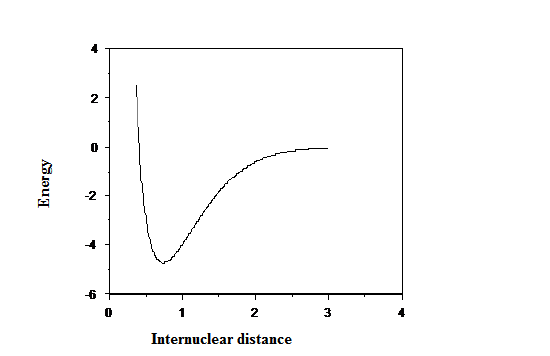
In the Morse potential function, \(D_e\) is the bond dissociation energy, \(r_e\) is the equilibrium bond length, and \(a\) is a constant that characterizes the steepness of the potential and thus affects the vibrational frequencies. The advantage of using the Morse potential to improve upon harmonic-oscillator-level predictions is that its energy levels and wave functions are also known exactly. The energies are given in terms of the parameters of the potential as follows:

\[E_n = \hbar \sqrt{\dfrac{k}{\mu}} { (n+\dfrac{1}{2}) - \dfrac{ (n+\dfrac{1}{2})^2\hbar \sqrt{k/\mu}}{4D_e} },\]

where the force constant is given in terms of the Morse potential’s parameters by \(k=2D_e a^2\). The Morse potential supports both bound states (those lying below the dissociation threshold for which vibration is confined by an outer turning point) and continuum states lying above the dissociation threshold (for which there is no outer turning point and thus the no spatial confinement). Its degree of anharmonicity is governed by the ratio of the harmonic energy \(\hbar \sqrt{\dfrac{k}{\mu}}\) to the dissociation energy \(D_e\).

The energy spacing between vibrational levels \(n\) and \(n+1\) are given by

\[E_{n+1} – E_n = \hbar \sqrt{\dfrac{k}{\mu}} \left( 1 - \dfrac{ (n+1)\hbar \sqrt{k/\mu}}{2D_e }\right).\]

These spacings decrease until \(n\) reaches the value \(n_{\rm max}\) at which

\[ { 1 - \dfrac{(n_{\rm max}+1) \hbar \sqrt{k/\mu}}{2D_e} } = 0,\]

after which the series of bound Morse levels ceases to exist (i.e., the Morse potential has only a finite number of bound states) and the Morse energy level expression shown above should no longer be used. It is also useful to note that, if \(\dfrac{\sqrt{2D_e\mu}}{a \hbar}\) becomes too small (i.e., < 1.0 in the Morse model), the potential may not be deep enough to support any bound levels. It is true that some attractive potentials do not have a large enough \(D_e\) value to have any bound states, and this is important to keep in mind. So, bound states are to be expected when there is a potential well (and thus the possibility of inner- and outer- turning points for the classical motion within this well) but only if this well is deep enough.

The eigenfunctions of the harmonic and Morse potentials display nodal character analogous to what we have seen earlier in the particle-in-boxes model problems. Namely, as the energy of the vibrational state increases, the number of nodes in the vibrational wave function also increases. The state having vibrational quantum number \(v\) has \(v\) nodes. I hope that by now the student is getting used to seeing the number of nodes increase as the quantum number and hence the energy grows. As the quantum number \(v\) grows, not only does the wave function have more nodes, but its probability distribution becomes more and more like the classical spatial probability, as expected. In particular for large-\(v\), the quantum and classical probabilities are similar and are large near the outer turning point where the classical velocity is low. They also have large amplitudes near the inner turning point, but this amplitude is rather narrow because the Morse potential drops off strongly to the right of this turning point; in contrast, to the left of the outer turning point, the potential decreases more slowly, so the large amplitudes persist over longer ranges near this turning point.

Contributors and Attributions

• Jack Simons (Henry Eyring Scientist and Professor of Chemistry, U. Utah) Telluride Schools on Theoretical Chemistry

• Integrated by Tomoyuki Hayashi (UC Davis)