1.3: The Born-Oppenheimer Approximation

One of the most important approximations relating to applying quantum mechanics to molecules and molecular ions is known as the Born-Oppenheimer (BO) approximation. The basic idea behind this approximation involves realizing that in the full electrons-plus-nuclei Hamiltonian operator introduced above

\[H = \sum_i \left[- \dfrac{\hbar^2}{2m_e} \dfrac{\partial^2}{\partial q_i^2} \right]+ \dfrac{1}{2} \sum_{j\ne i} \dfrac{e^2}{r_{i,j}} - \sum_{a,i} \dfrac{​Z_ae^2}{r_{i,a}} + \sum_a \left[- \dfrac{\hbar^2}{2m_a} \dfrac{\partial^2}{\partial q_a^2}\right]+ \dfrac{1}{2} \sum_{b\ne a} \dfrac{​Z_aZ_b e^2}{r_{a,b}} \]

the time scales with which the electrons and nuclei move are usually quite different. In particular, the heavy nuclei (i.e., even a H nucleus weighs nearly 2000 times what an electron weighs) move (i.e., vibrate and rotate) more slowly than do the lighter electrons. For example, typical bond vibrational motions occur over time scales of ca. \(10^{-14}\) s, molecular rotations require \(10^{-100}\) times as long, but electrons undergo periodic motions within their orbits on the \(10^{-17}\) s timescale if they reside within core or valence orbitals. Thus, we expect the electrons to be able to promptly “adjust” their motions to the much more slowly moving nuclei.

This observation motivates us to consider solving the Schrödinger equation for the movement of the electrons in the presence of fixed nuclei as a way to represent the fully adjusted state of the electrons at any fixed positions of the nuclei. Of course, we then have to have a way to describe the differences between how the electrons and nuclei behave in the absence of this approximation and how they move within the approximation. These differences give rise to so-called non-Born-Oppenheimer corrections, radiationless transitions, surface hops, and non-adiabatic transitions, which we will deal with later.

It should be noted that this separation of time scales between fast electronic and slow vibration and rotation motions does not apply as well to, for example, Rydberg states of atoms and molecules. As discussed earlier, in such states, the electron in the Rydberg orbital has much lower speed and much larger radial extent than for typical core or valence orbitals. For this reason, corrections to the BO model are usually more important to make when dealing with Rydberg states.

The electronic Hamiltonian that pertains to the motions of the electrons in the presence of clamped nuclei

\[H = \sum_i \left[- \dfrac{\hbar^2}{2m_e} \dfrac{\partial^2}{\partial q_i^2} \right]+ \dfrac{1}{2} \sum_{j\ne i} \dfrac{e^2}{r_{i,j}} - \sum_{a,i} \dfrac{​Z_ae^2}{r_{i,a}} \dfrac{1}{2} \sum_{b\ne a} \dfrac{​Z_a Z_b e^2}{r_{a,b}}\]

produces as its eigenvalues through the equation

\[H \psi_J(q_j|q_a) = E_J (q_a) \psi_J(q_j|q_a)\]

energies \(E_K (q_a)\) that depend on where the nuclei are located (i.e., the {\(q_a\)} coordinates). As its eigenfunctions, one obtains what are called electronic wave functions {\(\psi_K(q_i|q_a)\)} which also depend on where the nuclei are located. The energies \(E_K(q_a)\) are what we usually call potential energy surfaces. An example of such a surface is shown in Figure 1.5.

Figure 1.5. Two dimensional potential energy surface showing local minima, transition states and paths connecting them.

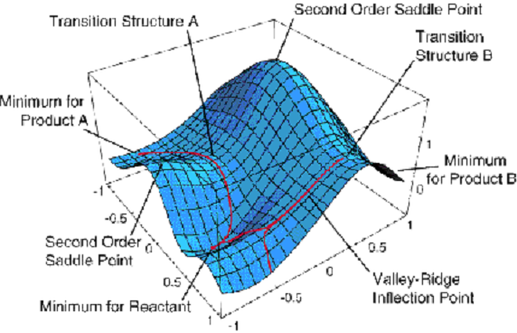
This surface depends on two geometrical coordinates \(\{q_a\}\) and is a plot of one particular eigenvalue \(E_J(q_a)\) vs. these two coordinates.

Although this plot has more information on it than we shall discuss now, a few features are worth noting. There appear to be three minima (i.e., points where the derivative of \(E_J\) with respect to both coordinates vanish and where the surface has positive curvature). These points correspond, as we will see toward the end of this introductory material, to geometries of stable molecular structures. The surface also displays two first-order saddle points (labeled transition structures A and B) that connect the three minima. These points have zero first derivative of \(E_J\) with respect to both coordinates but have one direction of negative curvature. As we will show later, these points describe transition states that play crucial roles in the kinetics of transitions among the three stable geometries.

Keep in mind that Figure 1.5 shows just one of the \(E_J\) surfaces; each molecule has a ground-state surface (i.e., the one that is lowest in energy) as well as an infinite number of excited-state surfaces. Let’s now return to our discussion of the BO model and ask what one does once one has such an energy surface in hand.

The motion of the nuclei are subsequently, within the BO model, assumed to obey a Schrödinger equation in which

\[\displaystyle\sum_a [- \dfrac{\hbar^2}{2m_a} \dfrac{\partial^2}{\partial q_a^2} ]+ \dfrac{1}{2} \sum_{b\ne a} \dfrac{Z_aZ_be^2}{r_{a,b}} + E_K(q_a)\]

defines a rotation-vibration Hamiltonian for the particular energy state \(E_K\) of interest. The rotational and vibrational energies and wave functions belonging to each electronic state (i.e., for each value of the index \(K\) in \(E_K(q_a)\)) are then found by solving a \(E_K\) Hamiltonian.

This BO model forms the basis of much of how chemists view molecular structure and molecular spectroscopy. For example as applied to formaldehyde \(H_2C=O\), we speak of the singlet ground electronic state (with all electrons spin paired and occupying the lowest energy orbitals) and its vibrational and rotational states as well as the \(n\rightarrow \pi^*\) and \(\pi\rightarrow \pi^*\) electronic states and their vibrational and rotational levels. Although much more will be said about these concepts later in this text, the student should be aware of the concepts of electronic energy surfaces (i.e., the {\(E_K(q_a)\)}) and the vibration-rotation states that belong to each such surface.

I should point out that the \(3N\) Cartesian coordinates {\(q_a\)} used to describe the positions of the molecule’s \(N\) nuclei can be replaced by 3 Cartesian coordinates \((X,Y,Z)\) specifying the center of mass of the \(N\) nuclei and \(3N-3\) other so-called internal coordinates that can be used to describe the molecule’s orientation (these coordinates appear in the rotational kinetic energy) and its bond lengths and angles (these coordinates appear in the vibrational kinetic and potential energies). When center-of-mass and internal coordinates are used in place of the \(3N\) Cartesian coordinates, the Born-Oppenheimer energy surfaces {\(E_K(q_a)\)} are seen to depend only on the internal coordinates. Moreover, if the molecule’s energy does not depend on its orientation (e.g., if it is moving freely in the gas phase), the {\(E_K(q_a)\)} will also not depend on the 3 orientational coordinates, but only on the \(3N-6\) vibrational coordinates.

Having been introduced to the concepts of operators, wave functions, the Hamiltonian and its Schrödinger equation, it is important to now consider several examples of the applications of these concepts. The examples treated below were chosen to provide the reader with valuable experience in solving the Schrödinger equation; they were also chosen because they form the most elementary chemical models of electronic motions in conjugated molecules and in atoms, rotations of linear molecules, and vibrations of chemical bonds.

Your First Application of Quantum Mechanics- Motion of a Particle in One Dimension

This is a very important problem whose solutions chemists use to model a wide variety of phenomena.

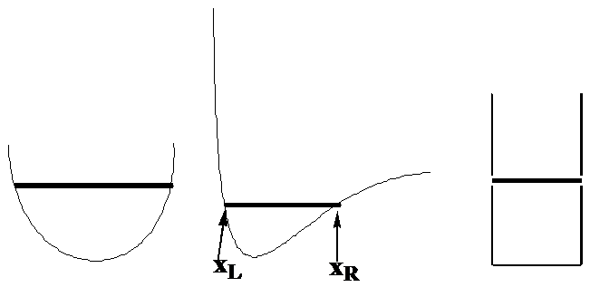
Let’s begin by examining the motion of a single particle of mass \(m\) in one direction which we will call \(x\) while under the influence of a potential denoted \(V(x)\). The classical expression for the total energy of such a system is \(E = \dfrac{p^2}{2m} + V(x)\), where \(p\) is the momentum of the particle along the x-axis. To focus on specific examples, consider how this particle would move if \(V(x)\) were of the forms shown in Figure 1. 6, where the total energy \(E\) is denoted by the position of the horizontal line.

Figure 1. 6. Three characteristic potentials showing left and right classical turning points at energies denoted by the horizontal lines.

The Classical Probability Density

I would like you to imagine what the probability density would be for this particle moving with total energy \(E\) and with \(V(x)\) varying as the above three plots illustrate. To conceptualize the probability density, imagine the particle to have a blinking lamp attached to it and think of this lamp blinking say 100 times for each time it takes for the particle to complete a full transit from its left turning point, to its right turning point and back to the former. The turning points \(x_L\) and \(x_R\) are the positions at which the particle, if it were moving under Newton’s laws, would reverse direction (as the momentum changes sign) and turn around. These positions can be found by asking where the momentum goes to zero:

\[0 = p = \sqrt{2m(E-V(x)}.\]

These are the positions where all of the energy appears as potential energy \(E = V(x)\) and correspond in the above figures to the points where the dark horizontal lines touch the \(V(x)\) plots as shown in the central plot.

The probability density at any value of \(x\) represents the fraction of time the particle spends at this value of \(x\) (i.e., within \(x\) and \(x+dx\)). Think of forming this density by allowing the blinking lamp attached to the particle to shed light on a photographic plate that is exposed to this light for many oscillations of the particle between \(x_L\) and \(x_R\). Alternatively, one can express the probability \(P(x) dx\) that the particle spends between \(x\) and \(x + dx\) by dividing the spatial distance \(dx\) by the velocity (p/m) of the particle at the point \(x\):

\[P(x)dx = \sqrt{2m(E-V(x))} \;m\; dx.\]

Because \(E\) is constant throughout the particle’s motion, \(P(x)\) will be small at \(x\) values where the particle is moving quickly (i.e., where \(V\) is low) and will be high where the particle moves slowly (where \(V\) is high). So, the photographic plate will show a bright region where \(V\) is high (because the particle moves slowly in such regions) and less brightness where \(V\) is low. Note, however, that as \(x\) approaches the classical turning points, the velocity approaches zero, so the above expression for \(P(x)\) will approach infinity. It does not mean the probability of finding the particle at the turning point is infinite; it means that the probability density is infinite there. This divergence of \(P(x)\) is a characteristic of the classical probability density that will be seen to be very different from the quantum probability density.

The bottom line is that the probability densities anticipated by analyzing the classical Newtonian dynamics of this one particle would appear as the histogram plots shown in Figure 1.7 illustrate.

Figure 1. 7 Classical probability plots for the three potentials shown

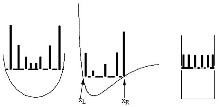
Where the particle has high kinetic energy (and thus lower \(V(x)\)), it spends less time and \(P(x)\) is small. Where the particle moves slowly, it spends more time and \(P(x)\) is larger. For the plot on the right, \(V(x)\) is constant within the “box”, so the speed is constant, hence \(P(x)\) is constant for all \(x\) values within this one-dimensional box. I ask that you keep these plots in mind because they are very different from what one finds when one solves the Schrödinger equation for this same problem. Also please keep in mind that these plots represent what one expects if the particle were moving according to classical Newtonian dynamics (which we know it is not!).

Quantum Treatment

To solve for the quantum mechanical wave functions and energies of this same kind of problem, we first write the Hamiltonian operator as discussed above by replacing \(p\) by \(-i\hbar \dfrac{d}{dx}\):

\[H = -\dfrac{ \hbar^2}{2m} \dfrac{d^2}{dx^2} + V(x).\]

We then try to find solutions \(\psi(x)\) to \(H\psi = E\psi\) that obey certain conditions. These conditions are related to the fact that \(|\psi (x)|^2\) is supposed to be the probability density for finding the particle between \(x\) and \(x+dx\). To keep things as simple as possible, let’s focus on the box potential \(V\) shown in the right side of Figure 1. 7. This potential, expressed as a function of \(x\) is: \(V(x) = \infty\) for \(x< 0\) and for \(x> L\); \(V(x) = 0\) for \(x\) between \(0\) and \(L\).

The fact that \(V\) is infinite for \(x< 0\) and for \(x> L\), and that the total energy \(E\) must be finite, says that \(\psi\) must vanish in these two regions (\(y = 0\) for \(x< 0\) and for \(x> L\)). This condition means that the particle cannot access regions of space where the potential is infinite. The second condition that we make use of is that \(\psi (x)\) must be continuous; this means that the probability of the particle being at \(x\) cannot be discontinuously related to the probability of it being at a nearby point. It is also true that the spatial derivative \(\dfrac{d\psi}{dx}\) must be continuous except at points where the potential \(V(x)\) has an infinite discontinuity like it does in the example shown on the right in Figure 1.7. The continuity of \(\dfrac{d\psi}{dx}\) relates to continuity of momentum (recall, \(-i \hbar \dfrac{\partial}{\partial x}\) is a momentum operator). When a particle moves under, for example, one of the two potential shown on the left or middle of Figure 1.7, the potential smoothly changes as kinetic and potential energy interchange during the periodic motion. In contrast, when moving under the potential on the right of Figure 1.7, the potential undergoes a sudden change of direction when the particle hits either wall. So, even classically, the particle’s momentum undergoes a discontinuity at such hard-wall turning points. These conditions of continuity of \(\psi\) (and its spatial first derivative) and that \(\psi\) must vanish in regions of space where the potential is extremely high were postulated by the pioneers of quantum mechanics so that the predictions of the quantum theory would be in line with experimental observations.

Energies and Wave functions

The second-order differential equation

\[- \dfrac{\hbar^2}{2m} \dfrac{d^2\psi}{dx^2} + V(x)\psi = E\psi\]

has two solutions (because it is a second order equation) in the region between \(x= 0\) and \(x= L\) where \(V(x) = 0\):

\[\psi = \sin(kx)\]

and

\[\psi = \cos(kx),\]

where \(k\) is defined as

\[k=\sqrt{2mE/\hbar^2}.\]

Hence, the most general solution is some combination of these two:

\[\psi = A \sin(kx) + B \cos(kx).\]

We could, alternatively use \(\exp(ikx)\) and \(\exp(-ikx)\) as the two independent solutions (we do so later in Section 1.4 to illustrate) because \(\sin(kx)\) and \(\cos(kx)\) can be rewritten in terms of \(\exp(ikx)\) and \(\exp(-ikx)\); that is, they span exactly the same space.

The fact that \(\psi\) must vanish at \(x= 0\) (n.b., \(\psi\) vanishes for \(x< 0\) because \(V(x)\) is infinite there and \(\psi\) is continuous, so it must vanish at the point \(x= 0\)) means that the weighting amplitude of the \(\cos(kx)\) term must vanish because \(\cos(kx) = 1\) at \(x = 0\). That is,

\[B = 0.\]

The amplitude of the \(\sin(kx)\) term is not affected by the condition that \(\psi\) vanish at \(x= 0\), since \(\sin(kx)\) itself vanishes at \(x= 0\). So, now we know that \(\psi\) is really of the form:

\[\psi(x) = A \sin(kx).\]

The condition that \(\psi\) also vanish at \(x= L\) (because it vanishes for \(x < 0\) where \(V(x)\) again is infinite) has two possible implications. Either \(A = 0\) or \(k\) must be such that \(\sin(kL) = 0\). The option \(A = 0\) would lead to an answer \(\psi\) that vanishes at all values of \(x\) and thus a probability that vanishes everywhere. This is unacceptable because it would imply that the particle is never observed anywhere.

The other possibility is that \(\sin(kL) = 0\). Let’s explore this answer because it offers the first example of energy quantization that you have probably encountered. As you know, the sin function vanishes at integral multiples of \(p\). Hence \(kL\) must be some multiple of \(\pi\); let’s call the integer \(n\) and write \(Lk = n\pi\) (using the definition of \(k\)) in the form:

\[L\sqrt{\dfrac{2mE}{\hbar^2}} = n\pi.\]

Solving this equation for the energy \(E\), we obtain:

\[E = \dfrac{n^2 \pi^2 \hbar^2}{2mL^2}\]

This result says that the only energy values that are capable of giving a wave function \(\psi (x)\) that will obey the above conditions are these specific \(E\) values. In other words, not all energy values are allowed in the sense that they can produce \(\psi\) functions that are continuous and vanish in regions where \(V(x)\) is infinite. If one uses an energy \(E\) that is not one of the allowed values and substitutes this \(E\) into \(\sin(kx)\), the resultant function will not vanish at \(x = L\). I hope the solution to this problem reminds you of the violin string that we discussed earlier. Recall that the violin string being tied down at \(x = 0\) and at \(x = L\) gave rise to quantization of the wavelength just as the conditions that \(\psi\) be continuous at \(x = 0\) and \(x = L\) gave energy quantization.

Substituting \(k = n\pi/L\) into \(\psi = A \sin(kx)\) gives

\[\psi (x) = A \sin\Big(\dfrac{np_x}{L}\Big).\]

The value of A can be found by remembering that \(|\psi|^2\) is supposed to represent the probability density for finding the particle at \(x\). Such probability densities are supposed to be normalized, meaning that their integral over all \(x\) values should amount to unity. So, we can find A by requiring that

\[1 = \int |\psi(x)|^2 dx = |A|^2 \int \sin^2\Big(\dfrac{np_x}{L}\Big)​dx\]​

where the integral ranges from \(x = 0\) to \(x = L\). Looking up the integral of \(\sin^2(ax)\) and solving the above equation for the so-called normalization constant \(A\) gives

\(A = \sqrt{\dfrac{2}{L}}\) and so

\[\psi(x) = \sqrt{\dfrac{2}{L}} \sin\Big(\dfrac{np_x}{L}\Big).\]

The values that \(n\) can take on are \(n = 1, 2, 3, \cdots\); the choice \(n = 0\) is unacceptable because it would produce a wave function \(\psi(x)\) that vanishes at all \(x\).

The full x- and t- dependent wave functions are then given as

\[\Psi(x,t) = \sqrt{\dfrac{2}{L}} \sin\Big(\dfrac{np_x}{L}\Big) \exp\bigg[-\dfrac{it}{\hbar}\dfrac{n^2 \pi^2\hbar^2}{2mL^2}\bigg].\]

Notice that the spatial probability density \(|\Psi(x,t)|^2\) is not dependent on time and is equal to \(|\psi(x)|^2\) because the complex exponential disappears when \(\Psi^*\Psi\) is formed. This means that the probability of finding the particle at various values of \(x\) is time-independent.

Another thing I want you to notice is that, unlike the classical dynamics case, not all energy values \(E\) are allowed. In the Newtonian dynamics situation, \(E\) could be specified and the particle’s momentum at any \(x\) value was then determined to within a sign. In contrast, in quantum mechanics, one must determine, by solving the Schrödinger equation, what the allowed values of \(E\) are. These \(E\) values are quantized, meaning that they occur only for discrete values \(E = \dfrac{n^2 \pi^2h^2}{2mL^2}\) determined by a quantum number \(n\), by the mass of the particle m, and by characteristics of the potential (\(L\) in this case).

Probability Densities

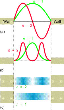
Let’s now look at some of the wave functions \(\psi (x)\) and compare the probability densities \(|\psi (x)|^2\) that they represent to the classical probability densities discussed earlier. The \(n=1\) and \(n=2\) wave functions are shown in the top of Figure 1.8. The corresponding quantum probability densities are shown below the wave functions in two formats (as \(x-y\) plots and shaded plots that could relate to the flashing light way of monitoring the particle’s location that we discussed earlier).

Figure 1. 8. The two lowest wave functions and probability densities

A more complete set of wave functions (for \(n\) ranging from 1 to 7) are shown in Figure 1. 9.

Figure 1. 9. Seven lowest wave functions and energies

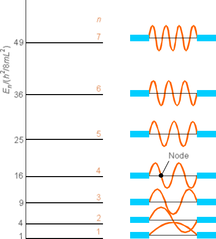
Notice that as the quantum number \(n\) increases, the energy \(E\) also increases (quadratically with \(n\) in this case) and the number of nodes in \(\psi\) also increases. Also notice that the probability densities are very different from what we encountered earlier for the classical case. For example, look at the \(n = 1\) and \(n = 2\) densities and compare them to the classical density illustrated in Figure 1.10.

Figure 1.10. Classical probability density for potential shown

The classical density is easy to understand because we are familiar with classical dynamics. In this case, we say that \(P(x)\) is constant within the box because the fact that \(V(x)\) is constant causes the kinetic energy and hence the speed of the particle to remain constant, and this is true for any energy \(E\). In contrast, the \(n = 1\) quantum wave function’s \(P(x)\) plot is peaked in the middle of the box and falls to zero at the walls. The \(n = 2\) density \(P(x)\) has two peaks (one to the left of the box midpoint, and one to the right), a node at the box midpoint, and falls to zero at the walls. One thing that students often ask me is “how does the particle get from being in the left peak to being in the right peak if it has zero chance of ever being at the midpoint where the node is?” The difficulty with this question is that it is posed in a terminology that asks for a classical dynamics answer. That is, by asking “how does the particle get...” one is demanding an answer that involves describing its motion (i.e., it moves from here at time \(t_1\) to there at time \(t_2\)). Unfortunately, quantum mechanics does not deal with issues such as a particle’s trajectory (i.e., where it is at various times) but only with its probability of being somewhere (i.e., \(|\psi|^2\)). The next section will treat such paradoxical issues even further.

Classical and Quantum Probability Densities

As just noted, it is tempting for most beginning students of quantum mechanics to attempt to interpret the quantum behavior of a particle in classical terms. However, this adventure is full of danger and bound to fail because small light particles simply do not move according to Newton’s laws. To illustrate, let’s try to understand what kind of (classical) motion would be consistent with the \(n = 1\) or \(n = 2\) quantum \(P(x)\) plots shown in Figure 1. 8. However, as I hope you anticipate, this attempt at gaining classical understanding of a quantum result will not work in that it will lead to nonsensical results. My point in leading you to attempt such a classical understanding is to teach you that classical and quantum results are simply different and that you must resist the urge to impose a classical understanding on quantum results at least until you understand under what circumstances classical and quantum results should or should not be comparable.

For the \(n = 1\) case in Figure 1.8, we note that \(P(x)\) is highest at the box midpoint and vanishes at \(x = 0\) and \(x = L\). In a classical mechanics world, this would mean that the particle moves slowly near \(x = \dfrac{L}{2}\) and more quickly near \(x = 0\) and \(x = L\). Because the particle’s total energy \(E\) must remain constant as it moves, in regions where it moves slowly, the potential it experiences must be high, and where it moves quickly, \(V\) must be small. This analysis (n.b., based on classical concepts) would lead us to conclude that the \(n =1\) \(P(x)\) arises from the particle moving in a potential that is high near \(x = \dfrac{L}{2}\) and low as \(x\) approaches 0 or L.

A similar analysis of the \(P(x)\) plot for \(n = 2\) would lead us to conclude that the particle for which this is the correct \(P(x)\) must experience a potential that is high midway between \(x = 0\) and \(x = \dfrac{L}{2}\), high midway between \(x = \dfrac{L}{2}\) and \(x = L\), and low near \(x = \dfrac{L}{2}\) and near \(x = 0\) and \(x = L\). These conclusions are crazy because we know that the potential \(V(x)\) for which we solved the Schrödinger equation to generate both of the wave functions (and both probability densities) is constant between \(x = 0\) and \(x = L\). That is, we know the same \(V(x)\) applies to the particle moving in the \(n = 1\) and \(n = 2\) states, whereas the classical motion analysis offered above suggests that \(V(x)\) is different for these two cases.

What is wrong with our attempt to understand the quantum \(P(x)\) plots? The mistake we made was in attempting to apply the equations and concepts of classical dynamics to a \(P(x)\) plot that did not arise from classical motion. simply put, one cannot ask how the particle is moving (i.e., what is its speed at various positions) when the particle is undergoing quantum dynamics. Most students, when first experiencing quantum wave functions and quantum probabilities, try to think of the particle moving in a classical way that is consistent with the quantum \(P(x)\). This attempt to retain a degree of classical understanding of the particle’s movement is almost always met with frustration, as I illustrated with the above example and will illustrate later in other cases.

Continuing with this first example of how one solves the Schrödinger equation and how one thinks of the quantized \(E\) values and wave functions \(\psi\), let me offer a little more optimistic note than offered in the preceding discussion. If we examine the \(\psi(x)\) plot shown in Figure 1.9 for \(n = 7\), and think of the corresponding \(P(x) = |\psi(x)|^2\), we note that the \(P(x)\) plot would look something like that shown in Figure 1. 11.

Figure 1.11. Quantum probability density for \(n = 7\) showing seven peaks and six nodes

It would have seven maxima separated by six nodes. If we were to plot \(|\psi(x)|^2\) for a very large \(n\) value such as \(n = 55\), we would find a \(P(x)\) plot having 55 maxima separated by 54 nodes, with the maxima separated approximately by distances of (1/55L). Such a plot, when viewed in a coarse-grained sense (i.e., focusing with somewhat blurred vision on the positions and heights of the maxima) looks very much like the classical \(P(x)\) plot in which \(P(x)\) is constant for all \(x\). Another way to look at the difference between the low-n and high-n quantum probability distributions is reflected in the so-called local de Broglie wavelength

\[\lambda_{\rm local}(x)=\dfrac{h}{\sqrt{2m(E-V(X))}}\]

It can be shown that the classical and quantum probabilities will be similar in regions of space where

\[\left|\dfrac{d\lambda_{\rm local}}{dx}\right| << 1.\]

This inequality will be true when \(E\) is much larger than \(V\), which is consistent with the view that high quantum states behave classically, but it will not hold when \(E\) is only slightly above \(V\) (i.e., for low-energy quantum states and for any quantum state near classical turning points) or when \(E\) is smaller than \(V\) (i.e., in classically forbidden regions).

In summary, it is a general result of quantum mechanics that the quantum \(P(x)\) distributions for large quantum numbers take on the form of the classical \(P(x)\) for the same potential \(V\) that was used to solve the Schrödinger equation except near turning points and in classically forbidden regions. It is also true that, at any specified energy, classical and quantum results agree better when one is dealing with heavy particles than for light particles. For example, a given energy \(E\) corresponds to a higher \(n\) quantum number in the particle-in-a-box formula \(E_n = \dfrac{n^2\hbar^2}{2mL^2}\) for a heavier particle than for a lighter particle. Hence, heavier particles, moving with a given energy \(E\), have more classical probability distributions.

To gain perspective about this matter, in the table shown below, I give the energy levels \(E_n = \dfrac{n^2\hbar^2}{2mL^2}\) in kcal mol^-1 for a particle whose mass is 1, 2000, 20,000, or 200,000 times an electron’s mass constrained to move within a one-dimensional region of length \(L\) (in Bohr units denoted \(a_0\); 1 \(a_0\) =0.529 Å).

Energies \(E_n\) (kcal mol^-1) for various \(m\) and \(L\) combinations

m = 1 m_e

	L = 1 a0	L = 10 a0	L = 100 a0	L = 1000 a0
m = 1 me	3.1 x10^3n^2	3.1 x10^1n^2	3.1 x10^-1n^2	3.1 x10^-3n^2
m = 2000 me	1.5 x10^0n^2	1.5 x10^-2n^2	1.5 x10^-4n^2	1.5 x10^-6n^2
m = 20,000 me	1.5 x10^-1n^2	1.5 x10^-3n^2	1.5 x10^-5n^2	1.5 x10^-7n^2
m = 200,000 me	1.5 x10^-2n^2	1.5 x10^-4n^2	1.5 x10^-6n^2	1.5 x10^-8n^2

Clearly, for electrons, even when free to roam over 50-500 nanometers (e.g., \(L = 100 a_0\) or \(L = 1000 a_0\)), one does not need to access a very high quantum state to reach 1 kcal mol^-1 of energy (e.g., \(n= 3\) would be adequate for \(L =100 a_0\)). Recall, it is high quantum states where one expects the classical and quantum spatial probability distribution to be similar. So, when treating electrons, one is probably (nearly) always going to have to make use of quantum mechanics and one will not be able to rely on classical mechanics.

For light nuclei, with masses near 2000 times the electron’s mass, if the particle is constrained to a small distance range (e.g., 1-10 \(a_0\)), again even low quantum states will have energies in excess of 1 kcal mol^-1. Only when free to move over of 100 to 1000 \(a_0\) does 1 kcal mol^-1 correspond to relatively large quantum numbers for which one expects near-classical behavior. The data shown in the above table can also be used to estimate when quantum behavior such as Bose-Einstein condensation can be expected. When constrained to 100 \(a_0\), particles in the 1 amu mass range have translational energies in the \(0.15 n^2\) cal mol^-1 range. Realizing that \(RT = 1.98\) cal mol^-1 K^-1, this means that translational temperatures near 0.1 K would be needed to cause these particles to occupy their \(n = 1\) ground state.

In contrast, particles with masses in the range of 100 amu, even when constrained

to distances of ca. 5 Å, require \(n\) to exceed ca. 10 before having 1 kcal mol^-1 of translational energy. When constrained to 50 Å, 1 kcal mol^-1 requires \(n\) to exceed 1000. So, heavy particles will, even at low energies, behave classically except if they are constrained to very short distances.

We will encounter this so-called quantum-classical correspondence principal again when we examine other model problems. It is an important property of solutions to the Schrödinger equation because it is what allows us to bridge the gap between using the Schrödinger equation to treat small light particles and the Newton equations for macroscopic (big, heavy) systems.

Time Propagation of Wave functions

For a particle in a box system that exists in an eigenstate \(\psi(x) = \sqrt{\dfrac{2}{L}} \sin\Big(\dfrac{np_x}{L}\Big)\) having an energy \(E_n = \dfrac{n^2 \pi^2\hbar^2}{2mL^2}\), the time-dependent wave function is

\[\Psi(x,t) = \sqrt{\dfrac{2}{L}} \sin\Big(\dfrac{np_x}{L}\Big) \exp\Big(-\dfrac{itE_n}{\hbar}\Big),\]

that can be generated by applying the so-called time evolution operator \(U(t,0)\) to the wave function at \(t = 0\):

\[\Psi(x,t) = U(t,0) \Psi(x,0),\]

where an explicit form for \(U(t,t’)\) is:

\[U(t,t’) = \exp\bigg[-\dfrac{i(t-t’)H}{\hbar}\bigg].\]

The function \(\Psi(x,t)\) has a spatial probability density that does not depend on time because

\[\Psi^*(x,t) \Psi(x,t) = \dfrac{2}{L} \sin^2\Big(\dfrac{np_x}{L}\Big) = \Psi^*(x,0) \Psi(x,0)\]

since \(\exp\Big(-\dfrac{itE_n}{\hbar}\Big) \exp\Big(\dfrac{itE_n}{\hbar}\Big) = 1\). However, it is possible to prepare systems (even in real laboratory settings) in states that are not single eigenstates; we call such states superposition states. For example, consider a particle moving along the x- axis within the box potential but in a state whose wave function at some initial time \(t = 0\) is

\[\Psi(x,0) = \dfrac{1}{\sqrt{2}} \sqrt{\dfrac{2}{L}} \sin\Big(\dfrac{1p_x}{L}\Big) – \dfrac{1}{\sqrt{2}} \sqrt{\dfrac{2}{L}} \sin\Big(\dfrac{2p_x}{L}\Big).\]

This is a superposition of the \(n =1\) and \(n = 2\) eigenstates. The probability density associated with this function is

\[|\Psi(x,0)|^2 = \dfrac{1}{2}\Big\{\dfrac{2}{L} \sin^2\Big(\dfrac{1p_x}{L}\Big)+ \dfrac{2}{L} \sin^2\Big(\dfrac{2p_x}{L}\Big) -2\dfrac{2}{L} \sin\Big(\dfrac{1p_x}{L}\Big)\sin\Big(\dfrac{2p_x}{L}\Big)\Big\}.\]

The \(n = 1\) and \(n = 2\) components, the superposition \(\Psi\), and the probability density at \(t = 0\) are shown in the first three panels of Figure 1.12.

Figure 1.12. The \(n = 1\) and \(n = 2\) wave functions (upper left), their superposition (upper right), and the \(t = 0\) (bottom left) and time-evolved (bottom right) probability densities of the superposition

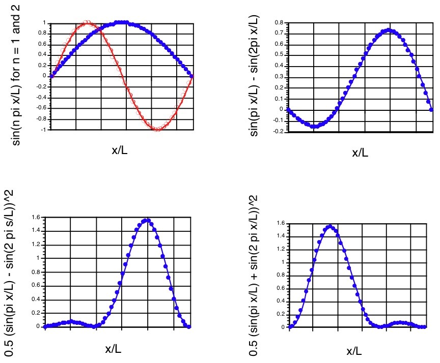
It should be noted that the probability density associated with this superposition state is not symmetric about the \(x=\dfrac{L}{2}\) midpoint even though the \(n = 1\) and \(n = 2\) component wave functions and densities are. Such a density describes the particle localized more strongly in the large-x region of the box than in the small-x region at \(t = 0\).

Now, let’s consider the superposition wave function and its density at later times. Applying the time evolution operator \(\exp\Big(-\dfrac{itH}{\hbar}\Big)\) to \(\Psi(x,0)\) generates this time-evolved function at time t:

\[\Psi(x,t) = \exp\Big(-\dfrac{itH}{\hbar}\Big) \left\{\dfrac{1}{\sqrt{2}} \sqrt{\dfrac{2}{L}} \sin\Big(\dfrac{1p_x}{L}\Big) – \dfrac{1}{\sqrt{2}} \sqrt{\dfrac{2}{L}} \sin\Big(\dfrac{2p_x}{L}\Big)\right\}\]

\[= {\dfrac{1}{\sqrt{2}} \sqrt{\dfrac{2}{L}} \sin\Big(\dfrac{1p_x}{L}\Big) \exp\Big(-\dfrac{itE_1}{\hbar}\Big) – \dfrac{1}{\sqrt{2}} \sqrt{\dfrac{2}{L}} \sin\Big(\dfrac{2p_x}{L}\Big) \exp\Big(-\dfrac{itE_2}{\hbar}\Big) }.\]

The spatial probability density associated with this \(\Psi\) is:

\[|\Psi(x,t)|^2 = \dfrac{1}{2}\Bigg\{\dfrac{2}{L} \sin^2\Big(\dfrac{1p_x}{L}\Big)+ \dfrac{2}{L} \sin^2\Big(\dfrac{2p_x}{L}\Big)-2\dfrac{2}{L} \cos\Big(\dfrac{(E_2-E_1)t}{\hbar}\Big) \sin\Big(\dfrac{1p_x}{L}\Big)\sin\Big(\dfrac{2p_x}{L}\Big)\Bigg\}.\]

At \(t = 0\), this function clearly reduces to that written earlier for \(\Psi(x,0)\). Notice that as time evolves, this density changes because of the \(\cos(E_2-E_1)\tau/\hbar\)) factor it contains. In particular, note that as \(t\) moves through a period of time \(\delta t = \dfrac{\pi\hbar}{E_2-E_1}\), the cos factor changes sign. That is, for \(t = 0\), the \(\cos\) factor is \(+1\); for \(t = \dfrac{\pi\hbar}{E_2-E_1}\), the cos factor is \(-1\); for \(t = \dfrac{2\pi\hbar}{E_2-E_1}\), it returns to \(+1\). The result of this time-variation in the cos factor is that \(|\Psi|^2\) changes in form from that shown in the bottom left panel of Figure 1. 12 to that shown in the bottom right panel (at \(t = \dfrac{\pi\hbar}{E_2-E_1}\)) and then back to the form in the bottom left panel (at \(t = \dfrac{2\pi\hbar}{E_2-E_1}\)). One can interpret this time variation as describing the particle’s probability density (not its classical position!), initially localized toward the right side of the box, moving to the left and then back to the right. Of course, this time evolution will continue over more and more cycles as time evolves further.

This example illustrates once again the difficulty with attempting to localize particles that are being described by quantum wave functions. For example, a particle that is characterized by the eigenstate \(\sqrt{\dfrac{2}{L}} \sin\Big(\dfrac{1p_x}{L}\Big)\) is more likely to be detected near \(x = \dfrac{L}{2}\) than near \(x = 0\) or \(x = L\) because the square of this function is large near \(x = \dfrac{L}{2}\). A particle in the state \(\sqrt{\dfrac{2}{L}} \sin\Big(\dfrac{2p_x}{L}\Big)\) is most likely to be found near \(x = \dfrac{L}{4}\) and \(x = \dfrac{3L}{4}\), but not near \(x = 0\), \(x = \dfrac{L}{2}\), or \(x =L\). The issue of how the particle in the latter state moves from being near \(x = \dfrac{L}{4}\) to \(x = \dfrac{3L}{4}\) is not something quantum mechanics deals with. Quantum mechanics does not allow us to follow the particle’s trajectory which is what we need to know when we ask how it moves from one place to another. Nevertheless, superposition wave functions can offer, to some extent, the opportunity to follow the motion of the particle.

For example, the superposition state written above as

\(\dfrac{1}{\sqrt{2}} \sqrt{\dfrac{2}{L}} \sin\Big(\dfrac{1p_x}{L}\Big) – \dfrac{1}{\sqrt{2}} \sqrt{\dfrac{2}{L}} \sin\Big(\dfrac{2p_x}{L}\Big)\) has a probability amplitude that changes with time as shown in Figure 1.12. Moreover, this amplitude’s major peak does move from side to side within the box as time evolves. So, in this case, we can say with what frequency the major peak moves back and forth. In a sense, this allows us to follow the particle’s movements, but only to the extent that we are satisfied with ascribing its location to the position of the major peak in its probability distribution. That is, we can not really follow its precise location, but we can follow the location of where it is very likely to be found. However, notice that the time it takes the particle to move from right to left \(t = \dfrac{\pi\hbar}{E_2-E_1}\) is dependent upon the energy difference between the two states contributing to the superposition state, not to the energy of either of these states, which is very different from what would expect if the particle were moving classically.

These are important observation that I hope the student will keep fresh in mind. They are also important ingredients in modern quantum dynamics in which localized wave packets, which are similar to superposed eigenstates discussed above, are used to detail the position and speed of a particle’s main probability density peak.

The above example illustrates how one time-evolves a wave function that is expressed as a linear combination (i.e., superposition) of eigenstates of the problem at hand. There is a large amount of current effort in the theoretical chemistry community aimed at developing efficient approximations to the \(\exp\Big(-\dfrac{itH}{\hbar}\Big)\) evolution operator that do not require \(\Psi(x,0)\) to be explicitly written as a sum of eigenstates. This is important because, for most systems of direct relevance to molecules, one can not solve for the eigenstates; it is simply too difficult to do so. You can find a significantly more detailed treatment of the research-level treatment of this subject in my Theory Page web site and my QMIC textbook. However, let’s spend a little time on a brief introduction to what is involved.

The problem is to express \(\exp\Big(-\dfrac{itH}{\hbar}\Big) \Psi(q_j)\), where \(\Psi(q_j)\) is some initial wave function but not an eigenstate, in a manner that does not require one to first find the eigenstates {\(\psi_J\)} of \(H\) and to expand \(\Psi\) in terms of these eigenstates:

\[\Psi (t=0) = \sum_J C_J \psi_J\]

after which the desired function is written as

\[\exp\Big(-\dfrac{itH}{\hbar}\Big) \Psi(q_j) = \sum_J C_J \psi_J \exp\Big(-\dfrac{itE_J}{\hbar}\Big).\]

The basic idea is to break the operator \(H\) into its kinetic \(T\) and potential \(V\) energy components and to realize that the differential operators appear in \(T\) only. The importance of this observation lies in the fact that \(T\) and \(V\) do not commute which means that \(TV\) is not equal to \(VT\) (n.b., recall that for two quantities to commute means that their order of appearance does not matter). Why do they not commute? Because \(T\) contains second derivatives with respect to the coordinates {q_j} that \(V\) depends on, so, for example, \(\dfrac{d^2}{dq^2}(V(q) \Psi(q))\) is not equal to \(V(q)\dfrac{d^2}{dq^2}\Psi(q)\). The fact that \(T\) and \(V\) do not commute is important because the most obvious attempt to approximate \(\exp\Big(-\dfrac{itH}{\hbar}\Big)\) is to write this single exponential in terms of \(\exp\Big(-\dfrac{itT}{\hbar}\Big)\) and \(\exp\Big(-\dfrac{itV}{\hbar}\Big)\). However, the identity

\[\exp\Big(-\dfrac{itH}{\hbar}\Big) = \exp\Big(-\dfrac{itV}{\hbar}\Big) \exp\Big(-\dfrac{itT}{\hbar}\Big)\]

is not fully valid as one can see by expanding all three of the above exponential factors as \(\exp(x) = 1 + x + \dfrac{x^2}{2!} + \cdots,\) and noting that the two sides of the above equation only agree if one can assume that \(TV = VT\), which, as we noted, is not true.

In most modern approaches to time propagation, one divides the time interval \(t\) into many (i.e., \(P\) of them) small time slices \(\tau = t/P\). One then expresses the evolution operator as a product of \(P\) short-time propagators (the student should by now be familiar with the fact that \(H\), \(T\), and \(V\) are operators, so, from now on I will no longer necessarily use bold lettering for these quantities):

\[\exp\Big(-\dfrac{itH}{\hbar}\Big) = \exp\Big(-\dfrac{i\tau H}{\hbar}\Big) \exp\Big(-\dfrac{i\tau H}{\hbar}\Big) \exp\Big(-\dfrac{i\tau H}{\hbar}\Big) \cdots = \left[\exp\Big(-\dfrac{i\tau H}{\hbar}\Big) \right]^P.\]

If one can then develop an efficient means of propagating for a short time \(\tau\), one can then do so over and over again \(P\) times to achieve the desired full-time propagation.

It can be shown that the exponential operator involving \(H\) can better be approximated in terms of the \(T\) and \(V\) exponential operators as follows:

\[\exp\Big(-\dfrac{i\tau H}{\hbar}\Big) \approx \exp\Big(-\dfrac{\tau^2 (TV-VT)}{\hbar^2}\Big) \exp\Big(-\dfrac{i\tau V}{\hbar}\Big) \exp\Big(-\dfrac{i\tau T}{\hbar}\Big).\]

So, if one can be satisfied with propagating for very short time intervals (so that the \(\tau^2\) term can be neglected), one can indeed use

\[\exp\Big(-\dfrac{i\tau H}{\hbar}\Big) \approx \exp\Big(-\dfrac{i\tau V}{\hbar}\Big) \exp\Big(-\dfrac{i\tau T}{\hbar}\Big)\]

as an approximation for the propagator \(U(t,0)\). It can also be shown that the so-called split short-time expression

\[\exp\Big(-\dfrac{i\tau H}{\hbar}\Big) \approx \exp\Big(-\dfrac{i\tau ​V}{2\hbar}\Big) \exp\Big(-\dfrac{i\tau T}{\hbar}\Big) \exp\Big(-\dfrac{i\tau ​V}{2\hbar}\Big) \]

provides an even more accurate representation of the short-time propagator (because expansions of the left- and right-hand sides agree to higher orders in \(\tau/\hbar\)).

To progress further, one then expresses \(\exp\Big(-\dfrac{i\tau T}{\hbar}\Big)\) acting on \(\exp\Big(-\dfrac{i\tau V}{2\hbar}\Big) \Psi(q)\) in terms of the eigenfunctions of the kinetic energy operator \(T\). Note that these eigenfunctions do not depend on the nature of the potential V, so this step is valid for any and all potentials. The eigenfunctions of \(T = - \dfrac{\hbar^2}{2m} \dfrac{d^2}{dq^2}\) are the momentum eigenfunctions that we discussed earlier

\[\psi_p(q) =\dfrac{1}{\sqrt{2\pi}} \exp\Big(\dfrac{ipq}{\hbar}\Big)\]

and they obey the following orthogonality

\[\int \psi_p'*(q) \psi_p(q) dq = d(p'-p)\]

and completeness relations

\[\int \psi_p(q) \psi_p^*(q') dp = d(q-q').\]

Writing \(\exp\Big(-\dfrac{i\tau V}{2\hbar}\Big) \Psi(q)\) as

\[\exp\Big(-\dfrac{i\tau ​V}{2\hbar}\Big)\Psi(q) = \int dq’ \delta(q-q') \exp\Big(-\dfrac{i\tau ​V(q’)}{2\hbar}\Big)\Psi(q'),\]

and using the above expression for \(\delta(q-q')\) gives:

\[\exp\Big(-\dfrac{i\tau ​V}{2\hbar}\Big)\Psi(q) = \int \int \psi_p(q) \psi_p^*(q') \exp\Big(-\dfrac{i\tau ​V(q’)}{2\hbar}\Big)\Psi(q') dq' dp.\]

Then inserting the explicit expressions for \(\psi_p(q)\) and \(\psi_p^*(q')\) in terms of

\[\psi_p(q) =\dfrac{1}{\sqrt{2\pi}} \exp\Big(\dfrac{ipq}{\hbar}\Big)\]

gives

\[\exp\Big(-\dfrac{i\tau V}{2\hbar}\Big)\Psi(q)\]

\[= \int \int\dfrac{1}{\sqrt{2\pi}} \exp\Big(\dfrac{ipq}{\hbar}\Big)\dfrac{1}{\sqrt{2\pi}} \exp\Big(-\dfrac{ipq'}{\hbar}\Big) \exp\Big(-\dfrac{i\tau V(q’)}{2\hbar}\Big)\Psi(q') dq' dp.\]

Now, allowing \(\exp\Big(-\dfrac{i\tau T}{\hbar}\Big)\) to act on \(\exp\Big(-\dfrac{i\tau V}{2\hbar}\Big) \Psi(q)\) produces

\[\exp\Big(-\dfrac{i\tau T}{\hbar}\Big) \exp\Big(-\dfrac{i\tau V}{2\hbar}\Big)\Psi(q) =\]

\[ \int \int \exp\Big(-\dfrac{i\tau\pi^2\hbar^2}{2m\hbar}\Big)\dfrac{1}{\sqrt{2\pi}} \exp\Big(-\dfrac{ip(q-q')}{\hbar}\Big)\dfrac{1}{\sqrt{2\pi}} \exp\Big(-\dfrac{i\tau V(q’)}{2\hbar}\Big)\Psi(q') dq' dp.\]

The integral over \(p\) above can be carried out analytically and gives

\[\exp\Big(-\dfrac{i\tau T}{\hbar}\Big) \exp\Big(-\dfrac{i\tau V}{2\hbar}\Big)\Psi(q) =\]

\[\sqrt{\dfrac{m}{2i\pi \tau\hbar}} \int \exp\Big(\dfrac{im(q-q')^2}{2\tau\hbar}\Big) \exp\Big(-\dfrac{i\tau V(q’)}{2\hbar}\Big) \Psi(q') dq'.\]

So, the final expression for the short-time propagated wave function is:

\[\Psi(q.t) = \sqrt{\dfrac{m}{2i\pi \tau\hbar}}\exp\Big(-\dfrac{i\tau V(q)}{2\hbar}\Big)\int \exp\Big(\dfrac{im(q-q')^2}{2\tau\hbar}\Big) \exp\Big(-\dfrac{i\tau V(q’)}{2\hbar}\Big)\Psi(q') dq',\]

which is the working equation one uses to compute \(\Psi(q,t)\) knowing \(\Psi(q)\). Notice that all one needs to know to apply this formula is the potential \(V(q)\) at each point in space. One does not need to know any of the eigenfunctions of the Hamiltonian to apply this method. This is especially attractive when dealing with very large molecules or molecules in condensed media where it is essentially impossible to determine any of the eigenstates and where the energy spacings between eigenstates is extremely small. However, one does have to use this formula over and over again to propagate the initial wave function through many small time steps \(\tau\) to achieve full propagation for the desired time interval \(t = P\tau\).

Because this type of time propagation technique is a very active area of research in the theory community, it is likely to continue to be refined and improved. Further discussion of it is beyond the scope of this book, so I will not go further into this direction. The web site of Professor Nancy Makri provides access to further information about the quantum time propagation research area.

Contributors and Attributions

• Jack Simons (Henry Eyring Scientist and Professor of Chemistry, U. Utah) Telluride Schools on Theoretical Chemistry

  Integrated by Tomoyuki Hayashi (UC Davis)