16.2: Raoult's Law and Ideal Solutions

An ideal solution is a homogeneous liquid solution that is at equilibrium with an ideal-gas solution in which the vapor pressure of each component satisfies Raoult’s law\({}^{1}\). Since the gas is ideal, the partial pressure of \(A\) is \(P_A=x_AP\). Raoult’s law asserts a relationship among the gas- and solution-phase mole fractions of \(A\), the vapor pressure of the pure liquid, and the pressure of the system:

\[P_A=x_AP=y_AP^{\textrm{⦁}}_A \nonumber \]

(Raoult’s law)

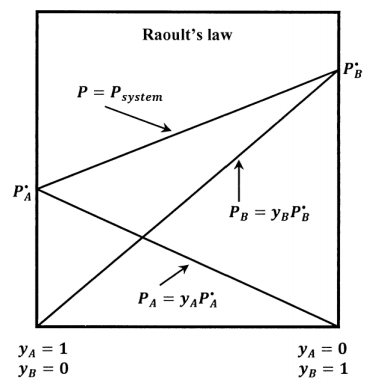
For a binary mixture of \(A\) and \(B\) that satisfies Raoult’s law, we have also that \(P_B=x_BP=y_BP^{\textrm{⦁}}_B\), and the total pressure becomes \(P=P_A+P_B=y_AP^{\textrm{⦁}}_A+y_BP^{\textrm{⦁}}_B\). The lines sketched in Figure 4 show how \(P_A\), \(P_B\), and \(P\) vary with the solution-phase composition when the solution is ideal.

Figure 4. Equilibrium pressures over an ideal solution.

When the standard state for \(A\) in solution is taken to be pure liquid \(A\) at its equilibrium vapor pressure, substitution of Raoult’s law into the results in Section 16.1 gives the activity of component \(A\) in an ideal solution as

\[{ \ln \left[{\tilde{a}}_A\left(P,y_A,y_B\right)\right]\ }={ \ln \left[\frac{x_AP}{P^{\textrm{⦁}}_A}\right]\ }={ \ln \left[\frac{y_AP^{\textrm{⦁}}_A}{P^{\textrm{⦁}}_A}\right]\ }={ \ln y_A\ } \nonumber \] and

\[{\tilde{a}}_A\left(P,y_A,y_B\right)=y_A \nonumber \]

(ideal solution, Raoult’s law)

In general, the activity and chemical potential of a component depend on pressure. If the solution is ideal, we see that the system pressure is fixed by \(P=y_AP^{\textrm{⦁}}_A+y_BP^{\textrm{⦁}}_B\), and the pure-component vapor pressures depend only on temperature. Since for the binary solution, \(y_B=1-y_A\), we can write the chemical potential of component \(A\) as

\[{\mu }_A\left(P,y_A,y_B\right)={\mu }_A\left(y_A\right)={\widetilde{\mu }}^o_A\left(\ell ,P^{\textrm{⦁}}_A\right)+RT{ \ln y_A\ } \nonumber \] (ideal solution)

We can also use relationships we develop earlier to find another representation for \({\widetilde{\mu }}^o_A\left(\ell ,P^{\textrm{⦁}}_A\right)\). The chemical potential of \(A\) in the liquid phase is the same as in the gas. Using the chemical potential for \(A\) in the gas phase that we find in Section 16.1, we have

\[{\mu }_A\left(P,y_A,y_B\right)={\mu }_A\left(g,P,x_A,x_B\right)={\Delta }_fG^o\left(A,{HIG}^o\right)+RT{ \ln \left[\frac{x_AP}{P^o}\right]\ }={\Delta }_fG^o\left(A,{HIG}^o\right)+RT{ \ln \left[\frac{P^{\textrm{⦁}}_A}{P^o}\right]\ }+RT{ \ln y_A\ } \nonumber \] and hence, \[{\widetilde{\mu }}^o_A\left(\ell ,P^{\textrm{⦁}}_A\right)={\Delta }_fG^o\left(A,{HIG}^o\right)+RT{ \ln \left[\frac{P^{\textrm{⦁}}_A}{P^o}\right]\ } \nonumber \]

In Section 15.4, we find, for an ideal gas,

\[{\Delta }_fG^o\left(A,{HIG}^o\right)+RT{ \ln \left[\frac{P^{\textrm{⦁}}_A}{P^o}\right]\ }={\Delta }_fG^o\left(A,\ell \right)+\int^{P^{\textrm{⦁}}_A}_{P^o}{{\overline{V}}^{\textrm{⦁}}_A\left(\ell \right)}dP \nonumber \]

so that the chemical potential of the pure liquid at its vapor pressure is also given by \[{\widetilde{\mu }}^o_A\left(\ell ,P^{\textrm{⦁}}_A\right)={\Delta }_fG^o\left(A,\ell \right)+\int^{P^{\textrm{⦁}}_A}_{P^o}{{\overline{V}}^{\textrm{⦁}}_A\left(\ell \right)}dP \nonumber \]

The integral is the difference between the Gibbs free energy of the pure liquid at its vapor pressure and that of the pure liquid at \(P^o=1\ \mathrm{bar}\). Note that we can obtain the same result much more simply by integrating \({\left(dG^{\textrm{⦁}}_A\right)}_T={\overline{V}}^{\textrm{⦁}}_AdP\) between the same two states. In Section 15.3, we see that the value of the integral is usually negligible. To a good approximation, we have

\[{\widetilde{\mu }}^o_A\left(\ell ,P^{\textrm{⦁}}_A\right)\approx {\Delta }_fG^o\left(A,\ell \right) \nonumber \]

(ideal solution)