3.8: A Heuristic View of the Cumulative Distribution Function

We can use these ideas to create a plot that approximates the cumulative probability distribution function given any set of \(N\) measurements of a random variable \(u\). To do so, we put the \(u_i\) values found in our \(N\) measurements in order from smallest to largest. We label the ordered values \(u_1\), \(u_2\),…,\(u_i\),…,\(u_N\), where \(u_1\) is the smallest. By the argument that we develop in the previous section, the probability of observing a value less than \(u_1\) is about \({1}/{\left(N+1\right)}\). If we were to make a large number of additional measurements, a fraction of about \({1}/{\left(N+1\right)}\) of this large number of additional measurements would be less than \(u_1\). This fraction is just \(f\left(u_1\right)\), so we reason that \(f\left(u_1\right)\approx {1}/{\left(N+1\right)}\). The probability of observing a value between \(u_1\) and \(u_2\) is also about \({1}/{\left(N+1\right)}\); so the probability of observing a value less than \(u_2\) is about \({2}/{\left(N+1\right)}\), and we expect \(f\left(u_2\right)\approx {2}/{\left(N+1\right)}\). In general, the probability of observing a value between \(u_{i-1}\) and \(u_i\) is also about \({1}/{\left(N+1\right)}\), and the probability of observing a value less than \(u_i\) is about \({i}/{\left(N+1\right)}\). In other words, we expect the cumulative probability distribution function for \(u_i\) to be such that the \(i^{th}\) smallest observation corresponds to \(f\left(u_i\right)\approx {i}/{\left(N+1\right)}\). The quantity \({i}/{\left(N+1\right)}\) is often called the rank probability of the \(i^{th}\) data point.

Figure 11. An approximate cumulative probability distribution function.

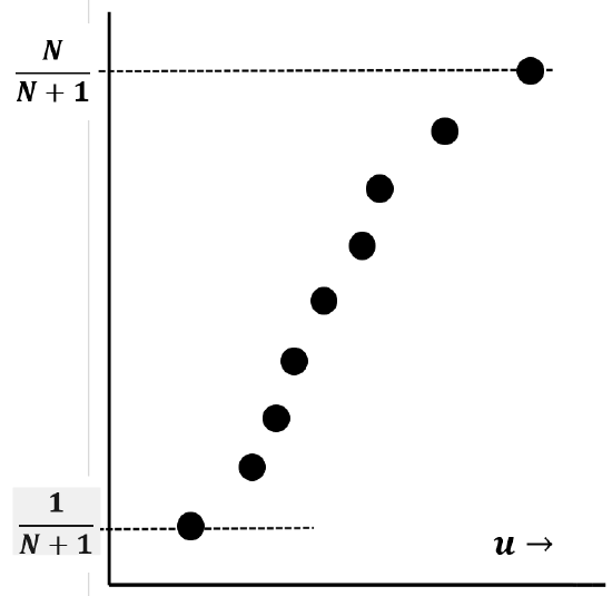
Figure 11 is a sketch of the sigmoid shape that we usually expect to find when we plot \({i}/{\left(N+1\right)}\) versus the \(i^{th}\) value of \(u\). This plot approximates the cumulative probability distribution function, \(f\left(u\right)\). We expect the sigmoid shape because we expect the observed values of \(u\) to bunch up around their average value. (If, within some domain of \(u\) values, all possible values of \(u\) were equally likely, we would expect the difference between successive observed values of \(u\) to be roughly constant, which would make the plot look approximately linear.) At any value of \(u\), the slope of the curve is just the probability-density function, \({df\left(u\right)}/{du}\).

These ideas mean that we can test whether the experimental data are described by any particular mathematical model, say \(F\left(u\right)\). To do so, we use the mathematical model to predict each of the N rank probability values: \({1}/{\left(N+1\right)}\), \({2}/{\left(N+1\right)}\),…, \({i}/{\left(N+1\right)}\),…, \({N}/{\left(N+1\right)}\). That is to say, we calculate \(F\left(u_1\right)\), \(F\left(u_2\right)\),…, \(F\left(u_i\right)\), …, \(F\left(u_N\right)\); if \(F\left(u\right)\) describes the data well, we will find, for all \(i\), \(F\left(u_i\right)\approx {i}/{\left(N+1\right)}\). Graphically, we can test the validity of the relationship by plotting \({i}/{\left(N+1\right)}\) versus \(F\left(u_i\right)\). If \(F\left(u\right)\) describes the data well, this plot will be approximately linear, with a slope of one.

In Section 3.12, we introduce the normal distribution, which is a mathematical model that describes a great many sources of experimental observations. The normal distribution is a distribution function that involves two parameters, the mean, \(\mu\), and the standard deviation, \(\sigma\). The ideas we have discussed can be used to develop a particular graph paper—usually called normal probability paper. If the data are normally distributed, plotting them on this paper produces an approximately straight line.

We can do essentially the same test without benefit of special graph paper, by calculating the average, \(\overline{u}\approx \mu\), and the estimated standard deviation, \(s\approx \sigma\), from the experimental data. (Calculating \(\overline{u}\) and \(s\) is discussed below.) Using \(\overline{u}\) and \(s\) as estimates of \(\mu\) and \(\sigma\), we can find the model-predicted probability of observing a value of the random variable that is less than \(u_i\). This value is \(f\left(u_i\right)\) for a normal distribution whose mean is \(\overline{u}\) and whose standard deviation is \(s\). We can find \(f\left(u_i\right)\) by using standard tables (usually called the normal curve of error in mathematical compilations), by numerically integrating the normal distribution’s probability density function, or by using a function embedded in a spreadsheet program, like Excel\({}^{\circledR }\). If the data are described by the normal distribution function, this value must be approximately equal to the rank probability; that is, we expect \(f\left(u_i\right)\approx {i}/{\left(N+1\right)}\). A plot of \({i}/{\left(N+1\right)}\) versus \(f\left(u_i\right)\) will be approximately linear with a slope of about one.