3.5: Bar Graphs and Histograms

Since a discrete distribution is completely specified by the probabilities of each of its events, we can represent it by a bar graph. The probability of each event is represented by the height of one bar. We can generalize this graphical representation to represent continuous distributions. To see what we have in mind, let us consider a particular example.

Let us suppose that we have a radar gun and that we decide to interest ourselves in the typical speeds of cars on a highway just outside of town. As we think about this project, we recognize that speeds might vary with the time of day and the day of the week. Random variations in many other factors might also be important; these include weather conditions and accidents in the vicinity. To eliminate as many atypical factors as possible, we might decide that typical speeds are those of cars going north between 1:00 pm and 4:00 pm on weekdays when the road surface is dry and there are no disabled vehicles in view. If we have a lot of time and the road is busy, we could collect a lot of data. Let us suppose that we record the speeds of \(10,000\) cars. Each datum would be the speed of a car on the road at a time when the selected conditions are satisfied.

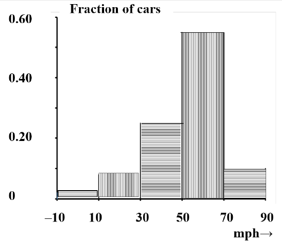
To use this data, we want to summarize it in a form that is easy to visualize. One way to do this is to aggregate the data to give the number of cars in each \(20\) mph range; the results might look something like the data in Table 2. Figure 3 is a five-channel bar graph that displays the number of cars in each \(20\) mph range. A great deal of information is lost in the aggregating process. In particular, nothing on the graph represents the number of automobiles in narrower speed intervals.

Table 2. Vehicle speed data.

Speed(mph)	Number of cars	Fraction of cars	Height for bar area to equal fraction
–10
	200	0.020	0.20/20 = 0.0010
10
	800	0.08	0.08/20 = 0.0040
30
	2500	0.25	0.25/20 = 0.0125
50
	5500	0.55	0.55/20 = 0.0275
70
	1000	0.10	0.10/20 = 0.0050
90

Now, suppose that we repeat this task, but that we do not have enough time to collect data on as many as \(10,000\) more cars. We will be curious about the extent to which our two samples agree with one another. Since the total number of vehicles will be different, the appropriate way to go about this is obviously to compare the fraction of cars in each speed range. In fact, using fractions enables us to compare any number of such studies. To the extent that these studies measure the same thing—typical speeds under the specified conditions—the fraction of automobiles in any particular speed interval should be approximately constant. Dividing the number of automobiles in each speed interval by the total number of automobiles gives a representation that focuses attention on the proportion of automobiles with various speeds. The shape of the bar graph remains the same; all that changes is the scale we use to label the ordinate. (See Figure 4.)

Figure 3. Number of cars versus speed.

Insofar as any repetition of this experiment gives nearly the same results, this is a useful change. However, the fundamental limitations of the graph remain. For example, if we want to use the graph to estimate how speeds are distributed in any other set of intervals, we have to read values off the ordinate and manipulate them in ways that may not be very satisfactory. To estimate the fraction with speeds between \(20\) mph and \(40\) mph, we might assign half of the automobiles in the \(10-30\) mph interval and half of those in the \(30-50\) mph interval to the new interval. This enables us to estimate that the fraction in the \(20-40\) mph interval is \(0.165\). This estimate is much less reliable than one that could be made by going back to the raw data for all \(10,000\) automobiles.

Figure 4. Fraction of cars versus speed.

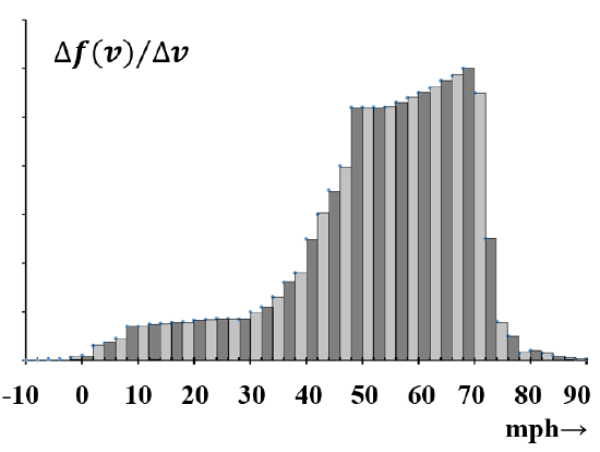
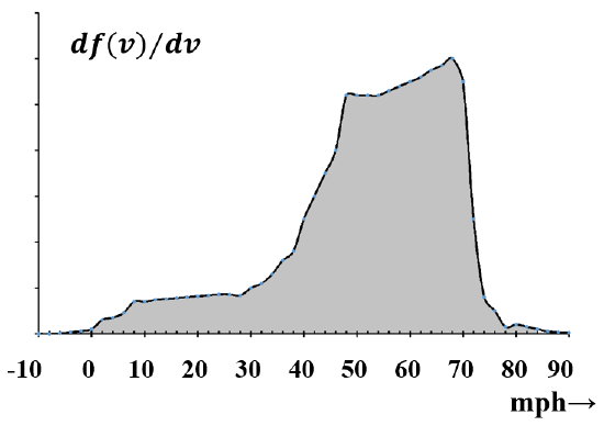
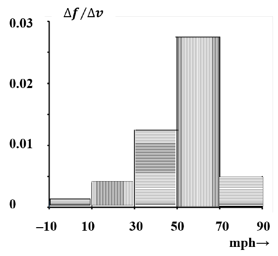
The data can also be represented as a histogram. In a histogram, the information is represented by the area rather than the height of the bar. In the present case, the only visible change to the graph is another change in the numerical values on the ordinate. In Figure 5, the area of a bar represents the fraction of automobiles with speeds in the given interval. As the speed interval is made smaller, any of these bar graphs looks increasingly like a continuous curve. (See Figure 6.) The histogram has the advantage that, as the curve becomes continuous, the interpretation remains constant: the area under the curve between any two speeds always represents the fraction of automobiles with speeds in this interval. It turns out that we are adept at visually estimating the relative areas of different parts of a histogram. That is, from a quick glance at a histogram, we are able to obtain a good semi-quantitative appreciation of the significance of the underlying data.

Figure 5. Speed data presented as a histogram.

If the histogram captures our experience, and we expect future events to have the same characteristics, the histogram becomes an expression of probability. All that is necessary is that we construct the histogram so that the total area under the graph is unity. If we let \(f\left(u\right)\) be the area under the graph from \(u=-\infty \) to \(u=u\), then \(f\left(u\right)\) represents the probability that the speed of a randomly selected automobile will lie between \(-\infty\) and \(u\). For any \(a\) and b, the probability that \(u\) lies in the interval \(a<b\)> is \(f\left(b\right)-f\left(a\right)\). The function \(f\left(u\right)\) is called the cumulative probability distribution function, because its value for any \(u\) is the fraction of automobiles that have a speed less than \(u\). \(f\left(a\right)\) is the frequency with which we observe values of the random variable, \(u\), that are less than \(a\). Equivalently, we can say that \(f\left(u\right)\) is the probability that any randomly selected automobile will have a speed less than \(u\). If we let the width of every interval go to zero, the bar graph representation of the histogram becomes a curve, and the histogram becomes a continuous function of the random variable, \(u\). (See Figure 7.) Note that the curve—the enclosing envelope—is not \(\boldsymbol{f}\left(\boldsymbol{u}\right)\).\(\boldsymbol{\ \ }\boldsymbol{f}\left(\boldsymbol{u}\right)\) is the area under the enclosing envelope curve.

Figure 6. Histogram with narrower speed intervals.

Figure 7. The histogram can be a continuous function.