4.7: Using Symmetry to Identify Integrals that are Zero

It generally requires much work and time to evaluate integrals analytically or even numerically on a computer. Our time, computer time, and work can be saved if we can identify by inspection when integrals are zero. The determination of when integrals are zero leads to spectroscopic selection rules and provides a better understanding of them. Here we use graphs to examine properties of the wavefunctions for a particle-in-a-box to determine when the transition dipole moment integral is zero and thereby obtain the spectroscopic selection rules for this system. These considerations are completely general and can be applied to any integrals. We essentially determine whether integrals are zero or not by drawing pictures and thinking. What could be easier?

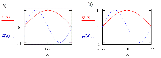
Consider the case for a transition from orbital \(n = 1\) to orbital \(n = 2\) of a molecule described by the particle-in-a-box model. These two wavefunctions are shown in Figure \(\PageIndex{1}\) as \(f1\) and \(f2\), respectively. For the curves shown on the left in the figure, we defined the box to have unit length, L = 1, and infinite potential barriers at \(x = 0\) and \(x = L\) as we did previously, so the particle is trapped between \(0\) and \(L\). For the curves shown on the right, \(g1\) and \(g2\), we put the origin of the coordinate system halfway between the potential barriers, i.e. at the center of the box. The barriers have not moved and the particle has not changed, but our description of the position of the barriers and the particle has changed. We now say the barriers are located at \(x = -L/2\) and \(x = +L/2\), and the particle is trapped between \(-L/2\) and \(+L/2\).

Clearly the wavefunctions in Figure \(\PageIndex{1}\) look the same for these two choices of coordinate systems. The appearance of the wavefunctions doesn’t depend on the coordinate system we have chosen or on our labels since the wavefunctions tell us about the probability of finding the particle. This probability does not change when we change the coordinate system or relabel the axis. The names of these functions do change, however. In Figure \(\PageIndex{1a}\), they both are sine functions. In Figure \(\PageIndex{1b}\), one is a cosine function and the other is a sine function multiplied by -1.

Figure \(\PageIndex{1}\): Wavefunctions for quantum state n=1 and quantum state n=2 in the two different coordinate systems.

Exercise \(\PageIndex{1}\)

Sketch \((f_1(x))^2\) and \((g_1(x))^2\). What do you observe? Sketch \((f_2(x))^2\) and \((g_2(x))^2\). What do you observe? What is the significance with respect to the probability given by both f(x) and g(x)?

We moved the origin of the coordinate system to the center of the box to take advantage of the symmetry properties of these functions. By symmetry, we mean the correspondence in form on either side of a dividing point, line, or plane. As we shall see, the analysis of the symmetry is straightforward if the origin of the coordinate systems coincides with the dividing point, line, or plane. Since the right and left halves of the box or molecule represented by the box are the same, the square of the wavefunction for x > 0 must be the same as the square of the wavefunction for x < 0. Since the box is symmetrical, the probability density, Ψ2, for the particle distribution also must be symmetrical because there is no reason for the particle to be located preferentially on one side or the other.

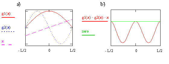
The transition moment integral for the particle-in-a-box involves three functions (\(ψ_f, ψ_i\), and x) that are multiplied together at each point x to form the integrand. These three functions for i = 1 and f = 2 are plotted on the left in Figure \(\PageIndex{2}\). The integrand is the product of these three functions and is shown on the right in the figure. The integral is the area between the integrand and the zero on the y-axis. Clearly this area and thus also the value of the integral is not zero. The integral is negative because \(ψ_2\) is negative for x > 0 and x is negative for x < 0. Since \(μ_T ≠ 0\), the transition from \(ψ_1\) to \(ψ_2\) is allowed. As we previously mentioned in this chapter, and will see again later, the absorption coefficient is proportional to the absolute square of \(μ_T\) so it is acceptable for the transition moment integral to be negative. It even could involve \(\sqrt {-1}\). Taking the absolute square makes both negative and imaginary quantities positive.

Figure \(\PageIndex{2}\): Functions (a) and integrand (b) of the transition moment integral for the transition from quantum state n = 1 to quantum state n = 2.

Exercise \(\PageIndex{2}\)

Write the expression or function for the integrand that is plotted on the right side of Figure \(\PageIndex{7}\) in terms of x, sine, and cosine functions. Use your function to explain why the integrand is 0 at x = 0 and has minima at x = + 0.25L and - 0.25L. Sketch the corresponding probability function.Where are the peaks in the probability function?

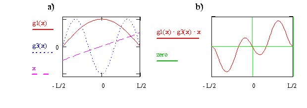
Now consider the transition moment integral for quantum state n = 1 to quantum state n = 3. In Figure \(\PageIndex{3}\), the wavefunctions and the x operator are shown on the left side, and the integrand is shown on the right side. For this case we see that the integrand for x < 0 is the negative of the integrand for x > 0. This difference in sign means the net positive area for x > 0 is canceled by the net negative area for x < 0, so the total area and the transition moment integral are zero. We therefore conclude that the transition from n = 1 to n = 3 is forbidden.

Figure \(\PageIndex{3}\): Functions (a) and integrand (b) of the transition moment integral for the transition from quantum state n = 1 to quantum state n = 3.

Exercise \(\PageIndex{3}\)

Write the expression or function for the integrand that is plotted on the right side of Figure \(\PageIndex{8}\) in terms of x and cosine functions. Use your function to explain why the integrand is zero at x = 0, why is it negative just above x = 0, and why as x goes from 0 to –0.5, the integrand first is positive and then negative.

In spectroscopy some special terms are used to describe the symmetry properties of wavefunctions. The terms symmetric, gerade, and even describe functions like \(f(x) = x^2\) and \(ψ_1(x)\) for the particle-in-a-box that have the property \(f(x) = f(-x)\), i.e. the function has the same values for x > 0 and for x < 0. The terms antisymmetric, ungerade, and odd describe functions like \(f(x) = x\) and \(ψ_2(x)\) for the particle-in-a-box that have the property \(f(x) = -f(-x)\), i.e. the function for \(x > 0\) is has values that are opposite in sign compared to the function for x < 0. Gerade and ungerade are German words meaning even and odd and are abbreviated as \(g\) and \(u\). Note that antisymmetric does not mean non-symmetric.

If an integrand is \(u\), then the integral is zero! It is zero because the contribution from \(x > 0\) is cancelled by the contribution from \(x < 0\), as shown by the example in Figure \(\PageIndex{8}\). An integrand will be u if the product of the functions comprising it is u. The following rules make it possible to quickly identify whether a product of two functions is u.

\[g \cdot g = g, u \cdot u = g, g \cdot u = u \label {4-33}\]

These rules are the same as those for multiplying +1 for \(g\) and -1 for \(u\). The validity of these rules can be seen by examining Figures \(\PageIndex{1}\) and \(\PageIndex{1}\). If an integrand consists of more than two functions, the rules are applied to pairs of functions to obtain the symmetry of their product, and then applied to pairs of the product functions, and so forth, until one obtains the symmetry of the integrand.

Exercise \(\PageIndex{4}\)

Use Mathcad or some other software to draw graphs of \(x^2, -x^2, x^3, and -x^3\) as a function of x. Which of these functions are g and which are u? Is the product function \(x^2 \cdot x^3 g\) or u? How about \(x^2 \cdot -x^2 \cdot x^3 \text {and} x^2 \cdot x^3 \cdot -x^3\)?

Exercise \(\PageIndex{5}\)

Label each function in Figures Figure \(\PageIndex{2}\) and Figure \(\PageIndex{3}\) as \(g\) or \(u\). Also label the integrands.

Exercise \(\PageIndex{6}\)

Use symmetry arguments to determine which of the following transitions between quantum states are allowed for the particle-in-a-box:

1. \(n = 2\) to \(n=3\)
2. \(n = 2\) to \(n=4\).

Symmetry properties of functions allow us to identify when the transition moment integral and other integrals are zero. This symmetry-based approach to integration can be generalized and becomes even more powerful when concepts taken from mathematical Group Theory are used. With the tools of Group Theory, one can examine symmetry properties in three-dimensional space for complicated molecular structures. A group-theoretical analysis helps understand features in molecular spectra, predict products of chemical reactions, and simplify theoretical calculations of molecular structures and properties.