
22.6.7: vi. Problem Solutions
- Page ID
- 85564

-
We will use the QMIC software to do this problem. Lets just start from the beginning. Get the starting "guess" mo coefficients on disk. Using the program MOCOEFS it asks us for the first and second mo vectors. We input 1, 0 for the first mo (this means that the first mo is 1.0 times the He 1s orbital plus 0.0 times the H 1s orbital; this bonding mo is more likely to be heavily weighted on the atom having the higher nuclear charge) and 0, 1 for the second. Our beginning mo-ao array looks like: \begin{bmatrix} 1.0 & 0.0 \\ 0.0 & 1.0 \end{bmatrix} and is placed on disk in a file we choose to call "mocoefs.dat". We also put the ao integrals on disk using the program RW_INTS. It asks for the unique one- and two- electron integrals and places a canonical list of these on disk in a file we choose to call "ao_integrals.dat". At this point it is useful for us to step back and look at the set of equations which we wish to solve: FC = SCE. The QMIC software does not provide us with a so-called generalized eigenvalue solver (one that contains an overlap matrix; or metric), so in order to use the diagonalization program that is provided we must transform this equation (FC = SCE) to one that looks like (F'C' = C'E). We do that in the following manner:
Since S is symmetric and positive definite we can find an \(S^{-\dfrac{1}{2}} \text{ such that } S^{-\dfrac{1}{2}} S^{+\dfrac{1}{2}} = 1, S^{-\dfrac{1}{2}} S = S^{+\dfrac{1}{2}}\),etc. rewrite FC = SCE by inserting unity between FC and multiplying the whole equation on the left by \( S^{-\dfrac{1}{2}} \). This gives:
\[ S^{-\dfrac{1}{2}} FS^{-\dfrac{1}{2}}S^{+\dfrac{1}{2}} C = S^{-\dfrac{1}{2}} SCE = S^{+\dfrac{1}{2}}CE \nonumber \]
Letting: \begin{align} F' &= S^{-\dfrac{1}{2}}FS^{-\dfrac{1}{2}} \\ C' &= S^{+\dfrac{1}{2}}C \text{, and inserting expressions above give: } \\ F'C' &= C'E \end{align}
Note, that to get the next iterations mo coefficients we must calculate C from C':
C' = \(S^{+\dfrac{1}{2}}\)C, so, multiplying through on the left by \(S^{-\dfrac{1}{2}}\) gives:
\[ S^{-\dfrac{1}{2}}C' = S^{-\dfrac{1}{2}}S^{+\dfrac{1}{2}}C = C \nonumber \]
This will be the method we will use to solve our fock equations.
Find \(S^{-\dfrac{1}{2}}\) by using the program FUNCT_MAT (this program generates a function of a matrix). This program will ask for the elements of the S array and write to disk a file (name of your choice ... a good name might be "shalf") containing the \(S^{-\dfrac{1}{2}}\) array. Now we are ready to begin the iterative Fock procedure.
a. Calculate the Fock matrix, F, using program FOCK which reads in the mo coefficients from "mocoefs.dat" and the integrals from "ao_integrals.dat" and writes the resulting Fock matrix to a user specified file (a good filename to use might be something like "fock1").
b. Calculate F' = \(S^{-\dfrac{1}{2}}FS^{-\dfrac{1}{2}}\) using the program UTMATU which reads in F and \(S^{-\dfrac{1}{2}}\) from files on the disk and writes F' to a user specified file (a good filename to use might be something like "fock1p"). Diagonalize F' using the program DIAG. This program reads in the matrix to be diagonalized from a user specified filename and writes the resulting eigenvectors to disk using a user specified filename (a good filename to use might be something like "coef1p"). You may wish to choose the option to write the eigenvalues (Fock orbital energies) to disk in order to use them at a later time in program FENERGY. Calculate C by back transforming e.g. C = \(S^{-\dfrac{1}{2}}\) C'. This is accomplished by using the program MATXMAT which reads in two matrices to be multiplied from user specified files and writes the product to disk using a user specified filename (a good filename to use might be something like "mocoefs.dat").
c. The QMIC program FENERGY calculates the total energy, using the result of exercises 2 and 3;
\[ \sum\limits_{kl} 2\langle k|h|k\rangle + 2\langle k1|1k \rangle - \langle k1|1k \rangle + \sum\limits_{\mu > \nu} \dfrac{Z_\mu Z_\nu}{R_{\mu\nu}} \text{, and } \sum\limits_k \varepsilon_k + \langle k|h|k \rangle + \sum\limits_{\mu > \nu }\dfrac{Z_\mu Z_\nu}{R_{\mu\nu}}. \nonumber \]
This is the conclusion of one iteration of the Fock procedure ... you may continue by going back to part a. and proceeding onward.
d. and e. Results for the successful convergence of this system using the supplied QMIC software is as follows (this is alot of bloody detail but will give the user assurance that they are on the right track; alternatively one could switch to the QMIC program SCF and allow that program to iteratively converge the Fock equations):
The one-electron AO integrals:
\[ \begin{bmatrix} -2.644200 & -1.511300 \\ -1.511300 & -1.720100 \end{bmatrix} \nonumber \]
The two-electron AO integrals:
\[ \begin{align} & 1 & & 1 & & 1 & & 1 & & 1.054700 & \\ & 2 & & 1 & & 1 & & 1 & & 0.4744000 & \\ & 2 & & 1 & & 2 & & 1 & & 0.5664000 & \\ & 2 & & 2 & & 1 & & 1 & & 0.2469000 & \\ & 2 & & 2 & & 2 & & 1 & & 0.3504000 & \\ & 2 & & 2 & & 2 & & 2 & & 0.6250000 & \end{align} \nonumber \]
The "initial" MO-AO coeffficients:
\[ \begin{bmatrix} 1.000000 & 0.000000 \\ 0.000000 & 1.000000 \end{bmatrix} \nonumber \]
AO overlap matrix (S):
\[ \begin{bmatrix} 1.000000 & 0.578400 \\ 0.578400 & 1.000000 \end{bmatrix} \nonumber \]
\[ S^{-\dfrac{1}{2}} \begin{bmatrix} 1.168032 & -0.3720709 \\ -0.3720709 & 1.168031 \end{bmatrix} \nonumber \]
************
ITERATION 1
************
The charge bond order matrix
\[ \begin{bmatrix} 1.000000 & 0.000000 \\ 0.000000 & 0.000000 \end{bmatrix} \nonumber \]
The Fock matrix (F):
\[ \begin{bmatrix} -1.589500 & -1.036900 \\ -1.036900 & -0.8342001 \end{bmatrix} \nonumber \]
\( S^{-\dfrac{1}{2}}FS^{-\dfrac{1}{2}} \)
\[ \begin{bmatrix} -1.382781 & -0.5048679 \\ -0.5048678 & -0.4568883 \end{bmatrix} \nonumber \]
The eigenvalues of this matrix (Fock orbital energies) are:
\[ [ -1.604825 -0.2348450 ] \nonumber \]
Their corresponding eigenvectors (C = \(S^{+\dfrac{1}{2}}*C\)) are:
\[ \begin{bmatrix} -0.9153809 & -0.4025888 \\ -0.4025888 & 0.9153810 \end{bmatrix} \nonumber \]
The "new" MO-AO coefficients (C = \(S^{-\dfrac{1}{2}}\)*C')
\[ \begin{bmatrix} -0.9194022 & -0.8108231 \\ -0.1296498 & 1.218985 \end{bmatrix} \nonumber \]
The one-electron MO integrals:
\[ \begin{bmatrix} -2.624352 & -0.1644336 \\ -0.1644336 & -1.306845 \end{bmatrix} \nonumber \]
The two-electron MO integrals:
\[ \begin{align} & 1 & & 1 & & 1 & & 1 & & 0.9779331 & \\ & 2 & & 1 & & 1 & &1 & & 0.1924623 & \\ & 2 & & 1 & & 2 & & 1 & & 0.5972075 & \\ & 2 & & 2 & & 1 & & 1 & & 0.1170838 & \\ & 2 & & 2 & & 2 & & 1 & & -0.0007945194 & \\ & 2 & & 2 & & 2 & & 2 & & 0.6157323 & \end{align} \nonumber \]
The closed shell Fock energy from formula:
\[ \sum\limits_{kl} 2 \langle k|h|k \rangle + 2\langle k1|k1 \rangle - \langle k1|1k \rangle + \sum\limits_{\mu >\nu} \dfrac{Z_\mu Z_\nu}{R_{\mu\nu}} = -2.84219933 \nonumber \]
from formula:
\[ \sum\limits_k \varepsilon_k + \langle k|h|k \rangle + \sum\limits_{\mu > \nu} \dfrac{Z_\mu Z_\nu}{R_{\mu\nu}} = -2.80060530 \nonumber \]
the difference is:
\[ -0.04159403 \nonumber \]
************
ITERATION 2
************
The change bond order matrix:
\[ \begin{bmatrix} 0.8453005 & 0.1192003 \\ 0.1192003 & 0.01680906 \end{bmatrix} \nonumber \]
The Fock matrix:
\[ \begin{bmatrix} -1.624673 & -1.083623 \\ -1.083623 & -0.8772071 \end{bmatrix} \nonumber \]
\( S^{-\dfrac{1}{2}}F S^{-\dfrac{1}{2}} \)
\[ \begin{bmatrix} -1.396111 & -0.5411037 \\ -0.5411037 & -0.4798213 \end{bmatrix} \nonumber \]
The eigenvalues of this matrix (Fock orbital energies) are:
\[ [ -1.646972 -0.2289599 ] \nonumber \]
Their corresponding eigenvectors (C' = \(S^{+\dfrac{1}{2}}\)*C) are:
\[ \begin{bmatrix} -0.9072427 & -0.4206074 \\ -0.4206074 & 0.9072427 \end{bmatrix} \nonumber \]
The "new" MO-AO coefficients (C = \(S^{-\dfrac{1}{2}}\)*C'):
\[ \begin{bmatrix} -0.9031923 & -0.8288413 \\ -0.1537240 & 1.216184 \end{bmatrix} \nonumber \]
The one-electron MO integrals:
\[ \begin{bmatrix} -2.617336 & -0.1903475 \\ -0.1903475 & -1.313861 \end{bmatrix} \nonumber \]
The two-electron MO integrals:
\[ \begin{align} & 1 & & 1 & & 1 & & 1 & & 0.9626070 & \\ & 2 & & 1 & & 1 & & 1 & & 0.1949828 & \\ & 2 & & 1 & & 2 & & 1 & & 0.6048143 & \\ & 2 & & 2 & & 1 & & 1 & & 0.1246907 & \\ & 2 & & 2 & & 2 & & 1 & & 0.003694540 & \\ & 2 & & 2 & & 2 & & 2 & & 0.6158437 & \end{align} \nonumber \]
The closed shell Fock energy from formula:
\[ \sum\limits_{kl} 2\langle k|h|k\rangle + 2\langle kl|kl \rangle - \langle kl|lk \rangle + \sum\limits_{\mu > \nu} \dfrac{Z_\mu Z_\nu}{R_{\mu\nu}} = -2.84349298 \nonumber \]
from formula:
\[ \sum\limits_k \varepsilon_k + \langle k|h|k \rangle + \sum\limits_{\mu > \nu} \dfrac{Z_\mu Z_\nu}{R_{\mu\nu}} = -2.83573675 \nonumber \]
the difference is:
\[ -0.00775623 \nonumber \]
************
ITERATION 3
************
The change bond order matrix:
\[ \begin{bmatrix} -1.631153 & -1.091825 \\ -1.091825 & -0.8853514 \end{bmatrix} \nonumber \]
\( S^{-\dfrac{1}{2}}FS^{-\dfrac{1}{2}} \)
\[ \begin{bmatrix} -1.398951 & -0.5470731 \\ -0.5470730 & -0.4847007 \end{bmatrix} \nonumber \]
The eigenvalues of this matrix (Fock orbital energies) are:
\[ [ -1.654745 -0.2289078 ] \nonumber \]
Their corresponding eigenvectors (C' = \(S^{+\dfrac{1}{2}}\)*C) are:
\[ \begin{bmatrix} -0.9058709 & -0.4235546 \\ -0.4235545 & 0.9058706 \end{bmatrix} \nonumber \]
The "new" MM-AO coefficients (C=S\( ^{-\dfrac{1}{2}} \)*C'):
\[ \begin{bmatrix} -0.9004935 & -0.8317733 \\ -0.1576767 & 1.215678 \end{bmatrix} \nonumber \]
The one-electron MO integrals:
\[ \begin{bmatrix} -2.616086 & -0.1945811 \\ -0.1945811 & -1.315112 \end{bmatrix} \nonumber \]
The two-electron MO integrals:
\[ \begin{align} & 1 & & 1 & & 1 & &1 & & 0.9600707 & \\ & 2 & & 1 & & 1 & & 1 & & 0.1953255 & \\ & 2 & & 1 & & 2 & & 1 & & 0.6060572 & \\ & 2 & & 2 & & 1 & & 1 & & 0.1259332 & \\ & 2 & & 2 & & 2 & & 1 & & 0.004475587 & \\ & 2 & & 2 & & 2 & & 2 & & 0.6158972 & \end{align} \nonumber \]
The closed shell Fock energy from formula:
\[ \sum\limits_{kl} 2\langle k|h|k\rangle + 2\langle kl|kl\rangle - \langle kl|lk\rangle + \sum\limits_{\mu > \nu} \dfrac{Z_\mu Z_\nu}{R_{\mu\nu }} = -2.84353018 \nonumber \]
from formula:
\[ \sum\limits_k \varepsilon_k + \langle k|h|k \rangle + \sum\limits_{\mu > \nu} \dfrac{Z_\mu Z_\nu}{R_{\mu\nu}} = -2.84225941 \nonumber \]
the difference is:
\[ -0.00127077 \nonumber \]
************
ITERATION 4
************
The charge bond order matrix:
\[ \begin{bmatrix} 0.8108885 & -1.093155 \\ -1.093155 & -0.8866909 \end{bmatrix} \nonumber \]
The Fock matrix:
\[ \begin{bmatrix} -1.632213 & -1.093155 \\ -1.093155 & -0.8866909 \end{bmatrix} \nonumber \]
\( S^{-\dfrac{1}{2}}FS^{-\dfrac{1}{2}} \)
\[ \begin{bmatrix} -1.399426 & -0.5480287 \\ -0.5480287 & -0.4855191 \end{bmatrix} \nonumber \]
The eigenvalues of this matrix (Fock orbital energies) are:
\[ [ -1.656015 -0.2289308 ] \nonumber \]
Their corresponding eigenvectors (C' = \(S^{+\dfrac{1}{2}}\)*C) are:
\[ \begin{bmatrix} -0.9056494 & -0.4240271 \\ -0.4240271 & 0.9056495 \end{bmatrix} \nonumber \]
The "new" MO-AO coefficients (C = \( S^{-\dfrac{1}{2}}\)*C'):
\[ \begin{bmatrix} -0.9000589 & -0.8322428 // -0.1583111 & 1.215595 \end{bmatrix} \nonumber \]
The one-electron MO integrals:
\[ \begin{bmatrix} -2.615881 & -0.1952594 \\ -0.1952594 & -1.315315 \end{bmatrix} \nonumber \]
The two-electron MO integrals:
\[ \begin{align} & 1 & & 1 & & 1 & & 1 & & 0.9596615 & \\ & 2 & & 1 & & 1 & & 1 & & 0.1953781 & \\ & 2 & & 1 & & 2 & & 1 & & 0.6062557 & \\ & 2 & & 2 & & 1 & & 1 & & 0.1261321 \\ & 2 & & 2 & & 2 & & 1 & & 0.004601604 & \\ & 2 & & 2 & & 2 & & 2 & & 0.6159065 & \end{align} \nonumber \]
The closed shell Fock energy from formula:
\[ \sum\limits_{kl} 2\langle k|h|k\rangle + 2\langle kl|kl\rangle - \langle kl|lk\rangle + \sum\limits_{\mu >\nu} \dfrac{Z_\mu Z_\nu}{R_{\mu\nu}} = -2.84352922 \nonumber \]
from formula:
\[ \sum\limits_k \varepsilon_k + \langle k|h|k\rangle + \sum\limits_{\mu >\nu} \dfrac{Z_\mu Z_\nu}{R_{\mu\nu}} = -2.84332418 \nonumber \]
the difference is:
\[ -0.00020504 \nonumber \]
************
ITERATION 5
************
The charge bond order matrix:
\[ \begin{bmatrix} 0.8101060 & 0.1424893 \\ 0.1424893 & 0.02506241 \end{bmatrix} \nonumber \]
The Fock matrix:
\[ \begin{bmatrix} -1.632385 & -1.093368 \\ -1.093368 & -0.8869066 \end{bmatrix} \nonumber \]
\( S^{-\dfrac{1}{2}}FS^{-\dfrac{1}{2}} \)
\[ \begin{bmatrix} -1.399504 & -0.5481812 \\ -0.5481813 & -0.4856516 \end{bmatrix} \nonumber \]
The eigenvalues of this matrix (Fock orbital energies) are:
\[ [ -1.656219 -0.2289360 ] \nonumber \]
Their corresponding eigenvectors (C' = S\(^{+\dfrac{1}{2}}\)*C) are:
\[ \begin{bmatrix} -0.9056138 & -0.4241026 \\ -0.4241028 & 0.9056141 \end{bmatrix} \nonumber \]
The "new" MO-AO coeficients (C = \(S^{-\dfrac{1}{2}}\)*C'):
\[ \begin{bmatrix} -0.8999892 & -0.8323179 \\ -0.1584127 & 1.215582 \end{bmatrix} \nonumber \]
The one-electron MO integrals:
\[ \begin{bmatrix} -2.615847 & -0.1953674 \\ -0.1953674 & -1.315348 \end{bmatrix} \nonumber \]
The two-electron MO integrals:
\[ \begin{align} & 1 & & 1 & & 1 & & 1 & & 0.9595956 & \\ & 2 & & 1 & & 1 & & 1 & & 0.1953862 & \\ & 2 & & 1 & & 2 & & 1 & & 0.6062872 & \\ & 2 & & 2 & & 1 & & 1 & & 0.1261639 & \\ & 2 & & 2 & & 2 & & 1 & & 0.004621811 & \\ & 2 & & 2 & & 2 & & 2 & & 0.6159078 & \end{align} \nonumber \]
The closed shell Fock energy from formula:
\[ \sum\limits_{kl} 2\langle k|h|k\rangle + 2\langle kl|kl\rangle - \langle kl|lk \rangle + \sum\limits_{\mu > \nu} \dfrac{Z_{\mu}Z_\nu}{R_{\mu\nu}} = -2.84352779 \nonumber \]
from formula:
\[ \sum\limits_k \varepsilon_k + \langle k|h|k\rangle + \sum\limits_{\mu > \nu} \dfrac{Z_\mu Z_\nu}{R_{\mu\nu}} = -2.84349489 \nonumber \]
the difference is:
-0.00003290
************
ITERATION 6
************
The charge bond order matrix:
\[ \begin{bmatrix} 0.8099805 & 0.1425698 \\ 0.1425698 & 0.02509460 \end{bmatrix} \nonumber \]
The Fock matrix:
\[ \begin{bmatrix} -1.632412 & -1.093402 \\ -1.093402 & -0.8869413 \end{bmatrix} \nonumber \]
\( S^{-\dfrac{1}{2}}FS^{-\dfrac{1}{2}} \)
\[ \begin{bmatrix} -1.399517 & -0.5482056 \\ -0.5482056 & -0.4856730 \end{bmatrix} \nonumber \]
The eigenvalues of this matrix (Fock orbital energies) are:
\[ [ -1.656253 -0.2289375 ] \nonumber \]
Their corresponding eigenvectors (C' = \(S^{+\dfrac{1}{2}}\)*C) are:
\[ \begin{bmatrix} -0.9056085 & -0.4241144 \\ -0.4241144 & 0.9056086 \end{bmatrix} \nonumber \]
The "new" MO-AO coefficients (C = \(S^{-\dfrac{1}{2}}\)*C'):
\[ \begin{bmatrix} 0.8999786 & -0.8323296 \\ -0.1584283 1.215580 \end{bmatrix} \nonumber \]
The one-electron MO integrals:
\[ \begin{bmatrix} -2.615843 & -0.1953846 \\ -0.1953846 & -1.315353 \end{bmatrix} \nonumber \]
The two-electron MO integrals:
\[ \begin{align} & 1 & & 1 & & 1 & & 1 & & 0.9595859 & \\ & 2 & & 1 & & 1 & & 1 & & 0.1953878 & \\ & 2 & & 1 & & 2 & & 1 & & 0.6062925 & \\ & 2 & & 2 & & 2 & & 1 & & 0.004625196 & \\ & 2 & & 2 & & 2 & & 2 & & 0.6159083 & \end{align} \nonumber \]
The closed shell Fock energy from formula:
\[ \sum\limits_{kl} 2\langle k|h|k\rangle 2 \langle kl|kl\rangle - \langle kl|lk\rangle + \sum\limits_{\mu >\nu} \dfrac{Z_\mu Z_\nu}{R_{\mu\nu}} = -2.84352827 \nonumber \]
from formula:
\[ \sum\limits_k \varepsilon_k + \langle k|h|k\rangle + \sum\limits_{\mu > \nu } \dfrac{Z_\mu Z_\nu}{R_{\mu\nu}} = -2.84352398 \nonumber \]
the difference is:
-0.00000429
************
ITERATION 7
************
The charge bond order matrix:
\[ \begin{bmatrix} 0.8099616 & 0.1425821 \\ 0.1425821 & 0.02509952 \end{bmatrix} \nonumber \]
The Fock matrix:
\[ \begin{bmatrix} -1.632416 & -1.093407 \\ -1.093407 & -0.8869464 \end{bmatrix} \nonumber \]
\( S^{-\dfrac{1}{2}}FS^{-\dfrac{1}{2}} \)
\[ \begin{bmatrix} -1.399519 & -0.5482093 \\ -0.5482092 & -0.4856761 \end{bmatrix} \nonumber \]
The eigenvalues of this matrix (Fock orbital energies) are:
\[ [ -1.656257 -0.2289374 ] \nonumber \]
Their corresponding eigenvectors (C' = \(S^{+\dfrac{1}{2}}\)*C) are:
\[ \begin{bmatrix} -0.9056076 & -0.4241164 \\ -0.4241164 & 0.9056077 \end{bmatrix} \nonumber \]
The "new" MO-AO coefficients (C=\(S^{-\dfrac{1}{2}}\)*C'):
\[ \begin{bmatrix} -0.8999770 & -0.8323317 \\ -0.1584310 & 1.215580 \end{bmatrix} \nonumber \]
The one-electron MO integrals:
\[ \begin{bmatrix} -2.615843 & -0.1953876 \\ -0.1953876 & -1.315354 \end{bmatrix} \nonumber \]
The two-electron MO integrals:
\[ \begin{align} & 1 & & 1 & & 1 & & 1 & & 0.9595849 & \\ & 2 & & 1 & & 1 & & 1 & & 0.1953881 & \\ & 2 & & 1 & & 2 & & 1 & & 0.6062936 & \\ & 2 & & 2 & & 1 & & 1 & & 0.1261697 & \\ & 2 & & 2 & & 2 & & 1 & & 0.004625696 & \\ & 2 & & 2 & & 2 & & 2 & & 0.6159083 & \end{align} \nonumber \]
The closed shell Fock energy from formula:
\[ \sum\limits_{kl} 2 \langle k|h|k\rangle + 2\langle kl|kl \rangle - \langle kl|lk \rangle + \sum\limits_{\mu > \nu} \dfrac{Z_\mu Z_\nu}{R_{\mu\nu}} = -2.84352922 \nonumber \]
from formula:
\[ \sum\limits_k \varepsilon_k + \langle k|h|k\rangle + \sum\limits_{\mu >\nu} \dfrac{Z_\mu Z_\nu}{R_{\mu\nu}} = -2.84352827 \nonumber \]
the difference is:
\[ -0.00000095 \nonumber \]
************
ITERATION 8
************
The charge bond order matrix:
\[ \begin{bmatrix} 0.8099686 & 0.1425842 \\ 0.1425842 & 0.02510037 \end{bmatrix} \nonumber \]
The Fock matrix:
\[ \begin{bmatrix} -1.632416 & -1.093408 \\ -1.093408 & -0.8869470 \end{bmatrix} \nonumber \]
\( S^{-\dfrac{1}{2}}FS^{-\dfrac{1}{2}} \)
\[ \begin{bmatrix} -1.399518 & -0.5482103 \\ -0.5482102 & -0.4856761 \end{bmatrix} \nonumber \]
The eigenvalues of this matrix (Fock orbital energies) are:
\[ [ -1.656258 -0.2289368 ] \nonumber \]
Their corresponding eigenvectors (C'=\(S^{+\dfrac{1}{2}}\)*C) are:
\[ \begin{bmatrix} -0.9056074 & -0.4241168 \\ -0.4241168 & 0.9056075 \end{bmatrix} \nonumber \]
The "new" MO-AO coefficients (C=\(S^{-\dfrac{1}{2}}\) *C'):
\[ \begin{bmatrix} -0.8999765 & -0.8323320 \\ -0.1584315 & 1.215579 \end{bmatrix} \nonumber \]
The one-electron MO integrals:
\[ \begin{bmatrix} -2.615842 & -0.1953882 \\ -0.1953882 & -1.315354 \end{bmatrix} \nonumber \]
The two-electron MO integrals:
\[ \begin{align} & 1 & & 1 & & 1 & & 1 & & 0.9595841 & \\ & 2 & & 1 & & 1 & & 1 & & 0.1953881 & \\ & 2 & & 1 & & 2 & & 1 & & 0.6062934 & \\ & 2 & & 2 & & 1 & & 1 & & 0.1261700 & \\ & 2 & & 2 & & 2 & & 1 & & 0.004625901 & \\ & 2 & & 2 & & 2 & & 2 & & 0.6159081 & \end{align} \nonumber \]
The closed shell Fock energy from formula:
\[ \sum\limits_{kl} 2\langle k|h|k\rangle + 2 \langle kl|kl\rangle - \langle kl|lk\rangle + \sum\limits_{\mu > \nu} \dfrac{Z_\mu Z_\nu}{R_{\mu\nu}} = -2.84352827 \nonumber \]
from formula:
\[ \sum\limits_k \varepsilon_k + \langle k|h|k\rangle + \sum\limits_{\mu >\nu} \dfrac{Z_\mu Z_\nu}{R_{\mu\nu}} = -2.84352827 \nonumber \]
the difference is:
\[ 0.00000000 \nonumber \]
f. In looking at the energy convergence we see the following:
Iteration Formula 1 Formula 2 1 -2.84219933 -2.80060530 2 -2.84349298 -2.83573675 3 -2.84353018 -2.84225941 4 -2.84352922 -2.84332418 5 -2.84352779 -2.84349489 6 -2.84352827 -2.84352827 7 -2.84352922 -2.84352827 8 -2.84352827 -2.84352827 f. If you look at the energy difference (SCF at iteration n - SCF converged) and plot this data versus iteration number, and do a 5th order polynomial fit, we see the following:
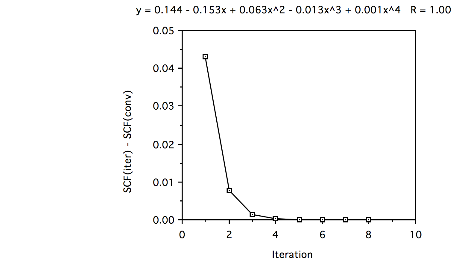
In looking at the polynomial fit we see that the convergence is primarily linear since the coefficient of the linear term is much larger than those of the cubic and higher terms.
g. The converged SCF total energy calculated using the result of exercise 3 is an upper bound to the ground state energy, but, during the iterative procedure it is not. At convergence, the expectation value of the Hamiltonian for the Hartree Fock determinant is given by the equation in exercise 3.
h. The one- and two- electron integrals in the MO basis are given above (see part e iteration 8). The orbital energies are found using the result of exercise 2 and 3 to be:
\begin{align} E(SCF) &= \sum\limits_k \varepsilon_k + \langle k|h|k\rangle + \sum\limits_{\mu > \nu} \dfrac{Z_\mu Z_\nu}{R_{\mu\nu}} \\ E(SCF) &= \sum\limits_{kl} 2\langle k|h|k \rangle + 2\langle kl|kl\rangle - \langle kl|lk\rangle + \sum\limits_{\mu > \nu} \dfrac{Z_\mu Z_\nu}{R_{\mu\nu}} \\ \text{so, } \varepsilon_k &= \langle k|h|k\rangle + \sum\limits_1^{occ} (2\langle kl|kl\rangle - \langle kl|lk\rangle ) \\ \varepsilon_1 &= h_{11} + 2\langle 11|11 \rangle - \langle 11|11\rangle \\ &= -2.615842 + 0.9595841 \\ &= -1.656258 \\ \varepsilon_2 &= h_{22} + 2\langle 21|21\rangle - \langle 21|12\rangle \\ &= -1.315354 + 2*0.6062934 - 0.1261700 \\ &= -0.2289372 \end{align}
i. Yes, the 1\(\sigma^2\) configuration does dissociate properly because at \( R\rightarrow \infty\) the lowest energy state is He + \(H^+\), which also has a \( 1\sigma^2\) orbital occupancy (i.e., \(1s^2\) on He and \(1s^0 \text{ on } H^+\)).
-
At convergence the mo coefficients are:
\[ \phi_1 = \begin{bmatrix} & -0.8999765 \\ & -0.1584315 \end{bmatrix} \phi_2 = \begin{bmatrix} & -0.8323320 \\ & 1.215579 \end{bmatrix} \nonumber \]
and the integrals in this MO basis are:
\begin{align} & h_{11} = -2.615842 & & h_{21} = -0.1953882 & & h_{22} = -1.315354 & \\ & g_{1111} = 0.9595841 & & g_{2111} = 0.1953881 & & g_{2121} = 0.6062934 & \\ & g_{2211} = 0.1261700 & & g_{2221} = 004625901 & & g_{2222} = 0.6159081 & \end{align}
a. \begin{align} H &= \begin{bmatrix} \langle 1\sigma^2|H|1\sigma^2\rangle & \langle 1\sigma^2|H|2\sigma^2\rangle \\ \langle 2\sigma^2|H|1\sigma^2\rangle & \langle 2\sigma^2|H|2\sigma^2\rangle \end{bmatrix} = \begin{bmatrix} 2h_{11} + g_{1111} & g_{1122} \\ g_{1122} & 2h_{22} + g_{2222} \end{bmatrix} \\ &= \begin{bmatrix} 2*-2.615842 + 0.9595841 & 0.1261700 \\ 0.126170 & 2*-1.315354 + 0.6159081 \end{bmatrix} \\ & = \begin{bmatrix} -4.272100 & 0.126170 \\ 0.126170 & -2.014800 \end{bmatrix} \end{align}
b. The eigenvalues are \(E_1 = -4.279131 \text{ and } E_2 = -2.007770.\) The corresponding eigenvectors are:
\[ C_1 = \begin{bmatrix} & -.99845123 \\ & 0.05563439 \end{bmatrix} \text{ , C_2 = } \begin{bmatrix} & 0.05563438 \\ & 0.99845140 \end{bmatrix} \nonumber \]
c. \begin{align} \dfrac{1}{2}&\left[ \bigg| \left(\sqrt{a}\phi_1 + \sqrt{b}\phi_2 \right) \alpha \left( \sqrt{a}\phi_1 - \sqrt{b}\phi_2\right)\beta\bigg| + \bigg|\left(\sqrt{a}\phi_1 - \sqrt{b}\phi_2\right)\alpha\left(\sqrt{a}\phi_1 + \sqrt{b}\phi_2\right)\beta\bigg| \right] \\ &= \dfrac{1}{2\sqrt{2}}\left[ \left( \sqrt{a}\phi_1 + \sqrt{b}\phi_2 \right)\left( \sqrt{a}\phi_1 - \sqrt{b}\phi_2 \right) + \left( \sqrt{a}\phi_1 - \sqrt{b}\phi_2 \right)\left( \sqrt{a}\phi_1 + \sqrt{b}\phi_2 \right) \right](\alpha\beta - \beta\alpha ) \\ &= \dfrac{1}{\sqrt{2}}(a\phi_1\phi_1 - b\phi_2\phi_2)(\alpha\beta - \beta\alpha) \\ &= a|\phi_1\alpha\phi_1\beta | - b|\phi_2\alpha\phi_2\beta |. & \text{(note from part b. a = 0.9984 and b = 0.0556)}\end{align}
d. The third configuration \( |1\sigma 2\sigma | = \dfrac{1}{\sqrt{2}} \left[ |1\alpha 2\beta | - | 1 \beta 2\alpha | \right]\),
Adding this configuration to the previous 2x2 CI results in the following 3x3 'full' CI:
\begin{align} H &= \begin{bmatrix} \langle 1\sigma^2 |H|1\sigma^2\rangle & \langle 1\sigma^2 |H|2\sigma^2\rangle & \langle 1\sigma^2 |H|1\sigma 2\sigma\rangle \\ \langle 2\sigma^2 |H|1\sigma^2\rangle & \langle 2\sigma^2 |H|2\sigma^2\rangle & \langle 2\sigma^2 |H|1\sigma 2\sigma\rangle \\ \langle 1\sigma 2\sigma |H|1\sigma^2\rangle & \langle 2\sigma^2 |H|1\sigma 2\sigma \rangle & \langle 1\sigma 2\sigma |H|1\sigma 2\sigma\rangle \end{bmatrix} \\ &= \begin{bmatrix} 2h_{11} + g_{1111} & g_{1122} & \dfrac{1}{\sqrt{2}}\left[ 2h_{12} + 2g_{2111}\right] \\ g_{1122} & 2h_{22} + g_{2222} & \dfrac{1}{\sqrt{2}}\left[ 2h_{12} + 2g_{2221}\right] \\ \dfrac{1}{\sqrt{2}}\left[ 2h_{12} + 2g_{2111}\right] & \dfrac{1}{\sqrt{2}}\left[ 2h_{12} + 2g_{2221}\right] & h_{11} + h_{22} + g_{2121} + g_{2211} \end{bmatrix} \end{align}
Evaluating the new matrix elements:
\begin{align} H_{12} &= H_{21} = \sqrt{2}*(-0.1953882 + 0.1953881) = 0.0 \\ H_{23} &= H_{32} = \sqrt{2}*(-0.1953882 + 0.004626) = -0.269778 \\ H_{33} &= -2.615842 - 1.315354 + 0.606293 + 0.126170 \\ &= -3.198733 \\ &= \begin{bmatrix} -4.272100 & 0.126170 & 0.0 \\ 0.126170 & -2.014800 & -0.269778 \\ 0.0 & -0.269778 & -3.198733 \end{bmatrix}\end{align}
e. The eigenvalues are \( E_1 = -4.279345 \text{, } E_2 = -3.256612 \text{ and } E_3 = -1.949678.\) The corresponding eigenvectors are:
\[ \begin{bmatrix} & -0.99825280 \\ & 0.05732290 \\ & 0.01431085 \end{bmatrix} \text{ , }C_2 = \begin{bmatrix} & -0.05302767 \\ & -0.20969283 \\ & -0.9774200 \end{bmatrix} \text{ , }C_3 = \begin{bmatrix} & -0.05302767 \\ & -0.97608540 \\ & 0.21082004 \end{bmatrix} \nonumber \]
f.We need the non-vanishing matrix elements of the dipole operator in the mo basis. These can be obtained by calculating them by hand. They are more easily obtained by using the TRANS program. Put the \(1e^-\) ao integrals on disk by running the program RW_INTS. In this case you are inserting \(z_{11} = 0.0 \text{, } z_{21} = 0.2854\text{, and } z_{22} = 1.4\) (insert 0.0 for all the \(2e^-\) integrals) ... call the output file "ao_dipole.ints" for example. The converged MO-AO coefficients should be in a file ("mocoefs.dat" is fine). The transformed integrals can be written to a file (name of your choice) for example "mo_dipole.ints". These matrix elements are:
\[ Z_{11} = 0.11652690 \text{, } z_{21} = -0.54420990 \text{, } z_{22} = 1.49117320 \nonumber \]
The excitation energies are \(E_2 - E_1 = -3.256612 - -4.279345 = 1.022733 \text{, and } E_3 - E_1 = -1.949678 .- - 4.279345 = 2.329667.\)
Using the Slater-Conden rules to obtain the matrix elements between configurations we get:
\begin{align} H_z &= \begin{bmatrix} \langle 1\sigma^2 |z| 1\sigma^2 \rangle & \langle 1\sigma^2 |z| 2\sigma^2 \rangle & \langle 1\sigma^2 |z| \sigma 2\sigma \rangle \\ \langle 2\sigma^2 |z| 1\sigma^2 \rangle & \langle 2\sigma^2 |z| 2\sigma^2 \rangle & \langle 2\sigma^2 |z| 1\sigma 2\sigma \rangle \\ \langle 1\sigma 2\sigma |z| 1\sigma^2 \rangle & \langle 2\sigma^2 |z| 1\sigma 2\sigma \rangle & \langle 1\sigma 2\sigma |z| 1\sigma 2\sigma \rangle \end{bmatrix} \\ &=\begin{bmatrix} 2z_{11} & 0 & \dfrac{1}{\sqrt{2}}\left[ 2z_{12}\right] \\ 0 & 2z_{22} & \dfrac{1}{\sqrt{2}}\left[ 2z_{12}\right] \\ \dfrac{1}{\sqrt{2}}\left[ 2z_{12}\right] & \dfrac{1}{\sqrt{2}}\left[ 2z_{12}\right] & z_{11} + z_{22} \end{bmatrix} \\ \begin{bmatrix} 0.233054 & 0 & -0.769629 \\ 0 & 2.982346 & -0.769629 \\ -0.769629 & -0.769629 & 1.607700 \end{bmatrix} \end{align}
Now, \( \langle \Psi_1 |z| \Psi_2 \rangle = C_1^TH_zC_2 \), (this can be accomplished with the program UTMATU)
\begin{align} &= \begin{bmatrix} &-0.99825280 \\ & 0.05732290 \\ & 0.01431085 \end{bmatrix}^T \begin{bmatrix} 0.233054 & 0 & -0.769629 \\ 0 & 2.982346 & -0.769629 \\ -0.769629 & -0.769629 & 1.607700 \end{bmatrix} \begin{bmatrix} & -0.02605343 \\ & -0.20969283 \\ & -0.9774200 \end{bmatrix} \\ &= -0.757494 \end{align}
and, \( \langle \Psi_1 |z| \Psi_3 \rangle = C_1^T H_zC_3\)
\begin{align} &= \begin{bmatrix} & -0.99825280 \\ & 0.05732290 \\ & 0.01431085 \end{bmatrix}^T \begin{bmatrix} 0.233054 & 0 & -0.769629 \\ 0 & 2.982346 & -0.769629 \\ -0.769629 & -0.769629 & 1.607700 \end{bmatrix} \begin{bmatrix} & -0.05302767 \\ & -0.97698540 \\ & 0.21082004 \end{bmatrix} \end{align}
g.Using the converged coefficients the orbital energies obtained from solving the Fock equations are \(\varepsilon_1 = -1.656258 \text{ and } \varepsilon_2 = -0.228938.\) The resulting expression for the RSPT first-order wavefunction becomes:
\begin{align} \big| 1\sigma^2 \rangle^{(1)} &= -\dfrac{g_{2211}}{2(\varepsilon_2 - \varepsilon_1 )}\big| 2\sigma^2\rangle \\ \big| 1\sigma^2\rangle^{(1)} &= -\dfrac{0.126170}{2( -0.228938 + 1.656258 )} \big|2\sigma^2\rangle \\ \big| 1\sigma^2\rangle^{(1)} &= -0.0441982\big| 2\sigma^2\rangle \end{align}
h. As you can see from part c., the matrix element \( \langle 1\sigma^2 |H| 1\sigma 2\sigma\rangle = 0\) (this is also a result of the Brillouin theorem) and hence this configuration does not enter into the first-order wavefunction.
i. \begin{align}& \big| 0\rangle = \big| 1\sigma^2\rangle - 0.0441982 \big| 2\sigma^2 \rangle . \text{To normalize we divide by:} \\ & \sqrt{\left[ 1 + (0.0441982)^2 \right]} = 1.0009762 \\ &\big|0\rangle = 0.999025\big| 1\sigma^2\rangle - 0.044155\big| 2\sigma^2\rangle \end{align}
In the 2x2 CI we obtained:
\begin{align} & \big|0\rangle = 0.99845123 \big| 1\sigma^2 \rangle - 0.05563439\big| 2\sigma^2\rangle \end{align}
j. The expression for the \(2^{nd}\) order RSPT is:
\begin{align} E^{(2)} &= -\dfrac{|g_{2211}|^2}{2(\varepsilon_2 - \varepsilon_1 )} = -\dfrac{0.126170^2}{2(-0.228938 + 1.656258)} \\ &= -0.005576 \text{ au } \end{align}
Comparing the 2x2 CI energy obtained to the SCF result we have:
-4.279131 - (-4.272102) = -0.007029 au
-
\begin{align} & \text{STO total energy: } & -2.8435283 \\ & \text{STO3G total energy } & -2.8340561 \\ & \text{ 3-21G total energy } & -2.8864405 \end{align}
The STO3G orbitals were generated as a best fit of 3 primitive gaussians (giving 1 CGTO) to the STO. So, STO3G can at best reproduce the STO result. The 3-21G orbitals are more flexible since there are 2 CGTOs per atom. This gives 4 orbitals (more parameters to optimize) and a lower total energy.
-
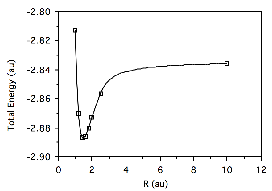
R \(HeH^+\) Energy \(H_2\) Energy 1.0
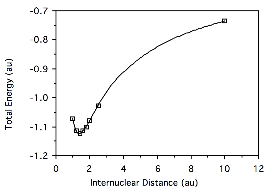
-2.812787056 -1.071953297 1.2 -2.870357513 -1.113775015 1.4 -2.886440516 -1.122933507 1.6 -2.886063576 -1.115567684 1.8 -2.880080938 -1.099872589 2.0 -2.872805595 -1.080269098 2.5 -2.856760263 -1.026927710 10.0 -2.835679293 -0.7361705303 Plotting total energy vs. geometry for \( HeH^+:\)
Plotting total energy vs. geometry for \(H_2:\)
For \(HeH^+\) at R = 10.0 au, the eigenvalues of the converged Fock matrix and the corresponding converged MO-AO coefficients are:
\begin{align} -0.1003571E+01 & -0.4961988E+00 & 0.5864846E+00 & 0.1981702E+01 \\ 0.4579189E+00 & -0.8245406E-05 & 0.1532163E-04 & 0.1157140E+01 \\ 0.6572777E+00 & -0.4580946E-05 & -0.6822942E-05 & -0.1056716E+01 \\ -0.1415438E-05 & 0.3734069E+00 & 0.1255539E+01 & -0.1669342E-04 \\ 0.1112778 & 0.71732444E+00 & -0.1096019E01 & 0.2031348E-04 \end{align}
Notice that this indicates that orbital 1 is a combination of the s functions on He only (dissociating properly to \( He + H^+\)).
For \(H_2 \text{ at } R = 10.0\) au, the eigenvalues of the converged Fock matrix and the corresponding converged MO-AO coefficients are:
\begin{align} -0.2458041E+00 & -0.1456223E+00 & 0.1137235E+01 & 0.1137825E+01 \\ 0.1977649E+00 & -0.1978204E+00 & 0.1006458E+01 & -0.7903225E+00 \\ 0.56325666E+00 & -0.5628273E+00 & -0.8179120E+00 & 0.6424941E+00 \\ 0.1976312E+00 & 0.1979216E+00 & 0.7902887E+00 & 0.1006491E+01 \\ 0.5629326E+00 & 0.5631776E+00 & -0.6421731E+00 & -0.6421731E+00 & -0.8181460E+00 \end{align}
Notice that this indicates that the orbital 1 is a combination of the s functions on both H atoms (dissociating improperly; equal probabilities of \(H_2\) dissociating to two neutral atoms or to a proton plus hydride ion).
- The \(H_2\) CI result"
R \(^1\sum_g^+\) \(^3\sum_u^+\) \(^1\sum_u^+\) \(^1\sum_g^+\) 1.0 -1.074970 -0.5323429 -0.3997412 0.3841676 1.2 -1.118442 -0.6450778 -0.4898805 0.1763018 1.4 -1.129904 -0.7221781 -0.5440346 0.0151913 1.6 -1.125582 -0.7787328 -0.5784428 -0.1140074 1.8 -1.113702 -0.8221166 -0.6013855 -0.2190144 2.0 -1.098676 -0.8562555 -0.6172761 -0.3044956 2.5 -1.060052 -0.9141968 -0.6384557 -0.4530645 5.0 -0.9835886 -0.9790545 -0.5879662 -0.5802447 7.5 -0.9806238 -0.9805795 -0.5247415 -0.5246646 10.0 -0.989598 -0.9805982 -0.4914058 -0.4913532 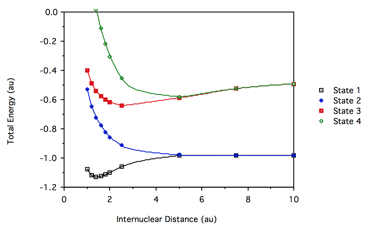
For \(H_2\) at R = 1.4 au, the eigenvalues of the Hamiltonian matrix and the corresponding determinant amplitudes are:
determinant -1.129904 -0.722178 -0.544035 0.015191 \( \big| 1\sigma_g\alpha 1\sigma_g \beta\big|\) 0.99695 0.00000 0.00000 0.07802 \( \big| 1\sigma_g\beta 1\sigma_u\alpha\big| \) 0.00000 0.70711 0.70711 0.00000 \( \big| 1\sigma_g\alpha 1\sigma_u\beta \big|\) 0.00000 0.70711 -0.70711 0.00000 \( \big| \sigma_u\alpha 1\sigma_u\beta\big| \) -0.07802 0.00000 0.00000 0.99695
This shows, as expected, the mixing of the first \( ^1\sum_g + (1\sigma_g^2 \text{ and the 2nd } ^1\sum_g^+ (1\sigma_u^2 )\) determinants, the
\[ ^3\sum\limits_u^+ = \left( \dfrac{1}{\sqrt{2}}\left( \big| 1\sigma_g\beta 1\sigma_u\alpha \big| + \big| 1\sigma_g\alpha 1\sigma_u\beta \big| \right) \right) , \nonumber \]
\[ \text{and the } ^1\sum\limits_u^+ = \left( \dfrac{1}{\sqrt{2}}\left( \big| 1\sigma_g\beta 1\sigma_u\alpha\big| - \big| 1\sigma_g\alpha 1\sigma_u\beta\big|\right) \right) . \nonumber \]
Also notice that the \( ^1\sum\limits_g^+\) state is the bonding (0.99695 - 0.07802) combination (note specifically the + - combination) and the second \(^1\sum\limits_g^+\) state is the antibonding combination (note specifically the + + combination). The + + combination always gives a higher energy than the + - combination. Also notice that the 1st and 2nd states \( (^1\sum\limits_g^+ \text{ and } ^3\sum\limits_u^+ )\) are dissociating to proton/anion combinations. The difference in these energies is the ionization potential of H minus the electron affinity of H.
- The \(H_2\) CI result"
-