
13.3: Anharmonicity
- Page ID
- 64793

The electronic energy of a molecule, ion, or radical at geometries near a stable structure can be expanded in a Taylor series in powers of displacement coordinates as was done in the preceding section of this Chapter. This expansion leads to a picture of uncoupled harmonic vibrational energy levels
\[ E(v_1 ... V_{3N - 5 \text{ or }6}) = \sum\limits_{j=1}^{3N-5 \text{ or }6}\hbar\omega _j\left( v_j + \frac{1}{2} \right) \nonumber \]
and wavefunctions
\[ \Psi(x_1 ... x_{3N-5\text{ or }6} = ^{3N-5 \text{ or }}_{j=1} \Psi_{vj}(x_j). \nonumber \]
The spacing between energy levels in which one of the normal-mode quantum numbers increases by unity
\[ \Delta E_{vj} = E(... v_j + 1 ... ) - E(...v_j ... ) = \hbar\omega_j \nonumber \]
is predicted to be independent of the quantum number vj . This picture of evenly spaced energy levels
\[ \Delta E_0 = \Delta E_1 = \Delta E_2 = ... \nonumber \]
is an incorrect aspect of the harmonic model of vibrational motion, and is a result of the quadratic model for the potential energy surface \(V(x_j).\)
The Expansion of E(v) in Powers of \(\left(v+\dfrac{1}{2}\right).\)
Experimental evidence clearly indicates that significant deviations from the harmonic oscillator energy expression occur as the quantum number \(v_j\) grows. In Chapter 1 these deviations were explained in terms of the diatomic molecule's true potential V(R) deviating strongly from the harmonic \( \frac{1}{2k}(E-E_e)^2 \) potential at higher energy (and hence larger \(|R-R_e|)\) as shown in the following figure.
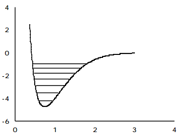
At larger bond lengths, the true potential is "softer" than the harmonic potential, and eventually reaches its asymptote which lies at the dissociation energy \(D_e\) above its minimum. This negative deviation of the true V(R) from \( \frac{1}{2k}(R-R_e)^2\) causes the true vibrational energy levels to lie below the harmonic predictions.
It is convention to express the experimentally observed vibrational energy levels, along each of the 3N-5 or 6 independent modes, as follows:
\[ E(v_j) = \hbar\left[ \omega_j\left(v_j + \frac{1}{2}\right) - (\omega x)_j \left(v_j + \frac{1}{2}\right)^2 + (\omega y)_j \left(v_j + \frac{1}{2}\right)^3 + (\omega z)_j \left( v_j + \frac{1}{2} \right)^4 + ... \right] \nonumber \]
The first term is the harmonic expression. The next is termed the first anharmonicity; it (usually) produces a negative contribution to E\((v_j)\) that varies as \( \left( v_j + \frac{1}{2} \right)^2 \). The spacings between successive \(v_j \rightarrow v_j + 1 \) energy levels is then given by:
\[ \Delta E_{vj} = E()v_j + 1) - E(v_j) \nonumber \]
\[ = \hbar [\omega_j - 2(\omega x)_j (v_j + 1) + ...] \nonumber \]
A plot of the spacing between neighboring energy levels versus \(v_j\) should be linear for values of vj where the harmonic and first overtone terms dominate. The slope of such a plot is expected to be \(-2\hbar(\omega x)_j\) and the small \(-v_j\) intercept should be \(\hbar[\omega_j - 2(\omega x)_j ].\) Such a plot of experimental data, which clearly can be used to determine the \(\omega_j \text{ and } (\omega x)_j\) parameter of the vibrational mode of study, is shown in the figure below.
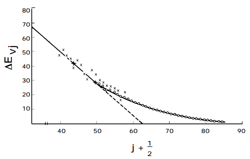
The Birge-Sponer Extrapolation
These so-called Birge-Sponer plots can also be used to determine dissociation energies of molecules. By linearly extrapolating the plot of experimental \(\Delta E_{vj}\) values to large vj values, one can find the value of \(v_j\) at which the spacing between neighboring vibrational levels goes to zero. This value \(v_j\), max specifies the quantum number of the last bound vibrational level for the particular potential energy function \(V(x_j)\) of interest. The dissociation energy \(D_e\) can then be computed by adding to \( \frac{1}{2}\hbar\omega _j \) (the zero point energy along this mode) the sum of the spacings between neighboring vibrational energy levels from \(v_j = 0 \text{ to } v_j = v_j,\text{ max }\):
\[ D_e \frac{1}{2}\hbar \omega_j + ^{v_j \text{ max }}_{v_j \text{ = 0 }}\Delta E_{v_j}. \nonumber \]
Since experimental data are not usually available for the entire range of \(v_j\) values (from 0 to \(v_j\),max), this sum must be computed using the anharmonic expression for \(\Delta E_{v_j}\) :
\[ \Delta E_{v_j} = \hbar \left[ \omega_j - 2(\omega x)_j \left( v_j + \dfrac{1}{2} + ... \right) \right]. \nonumber \]
Alternatively, the sum can be computed from the Birge-Sponer graph by measuring the area under the straight-line fit to the graph of \(\Delta E_{v_j} \text{ or } v_j \text{ from } v_j = 0 \text{ to } v_j = v_{j,\text{ max }}.\)
This completes our introduction to the subject of rotational and vibrational motions of molecules (which applies equally well to ions and radicals). The information contained in this Section is used again in Section 5 where photon-induced transitions between pairs of molecular electronic, vibrational, and rotational eigenstates are examined. More advanced treatments of the subject matter of this Section can be found in the text by Wilson, Decius, and Cross, as well as in Zare's text on angular momentum.