
4.3: Chemical Kinetics
- Page ID
- 106822

The term chemical kinetics refers to the study of the rates of chemical reactions. As we will see, differential equations play a central role in the mathematical treatment of chemical kinetics. We will start with the simplest examples, and then we will move to more complex cases. As you will see, in this section we will focus on a couple of reaction mechanisms. The common theme will be to find expressions that will allow us to calculate the concentration of the different species that take part of the reaction at different reaction times.
Let’s start with the simplest case, in which a reactant A reacts to give the product B. We’ll assume the reaction proceeds in one step, meaning there are no intermediates that can be detected.
\[\label{1order} A \overset{k}{\rightarrow}B\]
We’ll use the following notation for the time-dependent concentrations of A and B: [A]\((t)\), [B]\((t)\), or simply [A] and [B]. We’ll use [A]\(_0\) and [B]\(_0\) to denote the concentrations of A and B at time \(t=0\). The constant \(k\) is the rate constant of the reaction, and is a measure of how fast or slow the reaction is. It depends on the reaction itself (the chemical compounds A and B) and environmental factors such as temperature. The rate constant does not depend on the concentrations of the species involved in the reaction. The units of \(k\) depend on the particular mechanism of the reaction, as we will see through the examples. For the case described above, the units will be 1/time (e.g. \(s^{-1}\))
The rate of the reaction (\(r\)) will be defined as the number of moles of A that disappear or the number of moles of B that appear per unit of time (e.g. per second) and volume (e.g. liter). This is true because of the stoichiometry of the reaction, as we will discuss in a moment. However, because the rate is a positive quantity, we will use a negative sign if we look at the disappearance of A:
\[r=-\frac{d[A]}{dt}=\frac{d[B]}{dt}\]
The rate of the reaction, therefore, is a positive quantity with units of M.s\(^{-1}\), or in general, concentration per unit of time. As we will see, the rate of the reaction depends on the actual concentration of reactant, and therefore will in general decrease as the reaction progresses and the reactant is converted into product. Although all the molecules of A are identical, they do not need to react at the same instant. Consider the simple mechanism of Equation \ref{1order}, and imagine that every molecule of A has a probability \(p = 0.001\) of reacting in every one-second interval. Suppose you start with 1 mole of A in a 1 L flask (\([A]_0 = 1 M\)), and you measure the concentration of A one second later. How many moles of A do you expect to see? To answer this question, you can imagine that you get everybody in China (about one billion people) to throw a die at the same time, and that everybody who gets a six wins the game. How many winners do you expect to see? You know that the probability that each individual gets a six is \(p=1/6\), and therefore one-sixth of the players will win in one round of the game. Therefore, you can predict that the number of winers will be \(10^9/6\), and the number of losers will be \(5/6\times10^9\). If we get the losers to play a second round, we expect that one-sixth of them will get a six, which accounts for \(5/6\times10^9\times 1/6\) people. After the second run, therefore, we’ll still have \((5/6)^2\times10^9\) losers.
Following the same logic, the probability that a molecule of A reacts to give B in each one-second interval is \(= 1/1000\), and therefore in the first second you expect that \(6\times10^{23}/1000\) molecules react and \(999\times6\times10^{23}/1000\) remain unreacted. In other words, during the first second of your reaction 0.001 moles of A were converted into B, and therefore the rate of the reaction was \(10^{-3}Ms^{-1}\). During the second one-second interval of the reaction you expect that one-thousand of the remaining molecules will react, and so on. Imagine that you come back one hour later (3,600 s). We expect that \((999/1000)^{3,600}\times 6\times10^{23}\) molecules will remain unreacted, which is about \(1.6\times 10^{22}\) molecules. If you measure the reaction rate in the next second, you expect that one-thousand of them (\(1.6\times 10^{19}\) molecules, or \(2.7\times 10^{-5}\) moles) will react to give B. The rate of the reaction, therefore, decreased from \(10^{-3}Ms^{-1}\) at \(t=1s\) to \(2.7\times10^{-5}Ms^{-1}\) at \(t = 1h\). You should notice that the fraction of molecules of A that react in each one-second is always the same (in this case one-thousand). Therefore, the number of molecules that react per time interval is proportional to the number of molecules of A that remain unreacted at any given time. We just concluded that the rate of the reaction is proportional to the concentration of A:
\[\label{eq:1st} r=-\frac{d[A]}{dt}=\frac{d[B]}{dt}=k[A]\]
The proportionality constant, \(k\), is related to the probability that a molecule will react in a small time interval, as we discussed above. In this class, we will concentrate on solving differential equations such as the one above. This is a very simple differential equation that can be solved using different initial conditions. Let’s say that our goal is to find both [A]\((t)\) and [B]\((t)\). As chemists, we need to keep in mind that the law of mass conservation requires that
\[\label{mass} [A](t) + [B](t) = [A]_0 + [B]_0\]
In plain English, the concentrations of A and B at any time need to add up to the sum of the initial concentrations, as one molecule of A converts into B, and we cannot create or destroy matter. Again, keep in mind that this equation will need to be modified according to the stoichiometry of the reaction. We will call an equation of this type a ‘mass balance’.
Before solving this equation, let’s look at other examples. What are the differential equations that describe this sequential mechanism?
\[A \overset{k_1}{\rightarrow}B\overset{k_2}{\rightarrow}C \nonumber\]
In this mechanism, A is converted into C through an intermediate, B. Everything we discussed so far will apply to each of these two elementary reactions (the two that make up the overall mechanism). From the point of view of A nothing changes. Because the rate of the first reaction does not depend on B, it is irrelevant that B is converted into C (imagine you give 1 dollar per day to a friend. It does not matter whether you friend saves the money or gives it to someone else, you still lose 1 dollar per day).
\[\label{cons1} \frac{d[A]}{dt}=-k_1[A]\]
On the other hand, the rate of change of [B], \(d[B]/dt\) is the sum of the rate at which B is created (\(k_1[A]\)), minus the rate at which it disappears by reacting into C (\(k_2[B]\)):
\[\frac{d[B]}{dt}=k_1[A]-k_2[B] \label{cons2}\]
This can be read: The rate of change of [B] equals the rate at which [B] appears from A into B, minus the rate at which [B] disappears from B into C. In each term, the rate is proportional to the reactant of the corresponding step: A for the first reaction, and B for the second step.
What about C? Again, it is irrelevant that B was created from A (if you get 1 dollar a day from your friend, you don’t care if she got it from her parents, you still get 1 dollar per day). The rate at which C appears is proportional to the reactant in the second step: B. Therefore:
\[\frac{d[C]}{dt}=k_2[B] \label{cons3}\]
The last three equations form a system of differential equations that need to be solved considering the initial conditions of the problem (e.g. initially we have A but not B or C). We’ll solve this problem in a moment, but we still need to discuss a few issues related to how we write the differential equations that describe a particular mechanism. Imagine that we are interested in
\[2 A + B \overset{k}{\rightarrow}3 C \nonumber\]
We know that the rate of a reaction is defined as the change in concentration with time...but which concentration? is it \(d[A]/dt\)? or \(d[B]/dt\)? or \(d[C]/dt\)? These are all different because 3 molecules of C are created each time 1 of B and 2 of A disappear. Which one should we use? Because 2 of A disappear every time 1 of B disappears: \(d[A]/dt= 2 d[B]/dt\). Now, considering that rates are positive quantities, and that the derivatives for the reactants, \(d[A]/dt\) and \(d[B]/dt\), are negative:
\[r=-\frac{1}{2}\frac{d[A]}{dt}=-\frac{d[B]}{dt}=\frac{1}{3}\frac{d[C]}{dt}\]
This example shows how to deal with the stoichiometric coefficients of the reaction. Note that in all our examples we assume that the reactions proceed as written, without any ‘hidden’ intermediate steps.
First order reactions
We have covered enough background, so we can start solving the mechanisms we introduced. Let’s start with the easiest one (Equations \ref{1order}, \ref{eq:1st} and \ref{mass}):
\[A \overset{k}{\rightarrow}B \nonumber\]
\[r=-\frac{d[A]}{dt}=\frac{d[B]}{dt}=k[A] \nonumber\]
\[[A](t) + [B](t) = [A]_0 + [B]_0 \nonumber\]
This mechanism is called a first order reaction because the rate is proportional to the first power of the concentration of reactant. For a second-order reaction, the rate is proportional to the square of the concentration of reactant (see Problem \(4.3\)). Let’s start by finding \([A](t)\) from \(-\frac{d[A]}{dt}=k[A]\). We’ll then obtain\([B](t)\) from the mass balance. This is a very simple differential equation because it is separable:
\[-\frac{d[A]}{dt}=k[A] \nonumber\]
\[\frac{d[A]}{[A]}=-kdt \nonumber\]
We integrate both sides of the equation, and combine the two integration constants in one:
\[\ln{[A]}=-kt+c \nonumber\]
We need to solve for [A]:
\[[A]=e^{-kt+c}=e^ce^{-kt}=c_2e^{-kt} \nonumber\]
This is the general solution of the problem. Let’s assume we are giving the following initial conditions: [A]\((t=0)=[A]_0\), [B]\((t=0)=0.\) We’ll use this information to find the arbitrary constant \(c_2\):
\[[A](t=0)=c_2e^{0}=c_2 \nonumber\]
Therefore, the particular solution is:
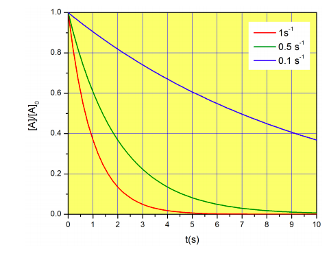
\[\label{eq:mdecay} [A](t)=[A]_0e^{-kt}\]
What about [B]? From the mass balance, [B] = [A]\(_0\) + [B]\(_0\) - [A] = [A]\(_0\) - [A]\(_0e^{-kt}= [A]_0\left(1-e^{-kt}\right)]\).
Figure \(\PageIndex{4}\) shows three examples of decays with different rate constants.
We can calculate the half-life of the reaction (\(t_{1/2}\)), defined as the time required for half the initial concentration of A to react. From Equation \ref{eq:mdecay}:
\[\frac{[A](t)}{[A]_0}=e^{-kt} \nonumber\]
When \(t=t_{1/2}\),
\[\frac{1}{2}=e^{-kt_{1/2}} \nonumber\]
\[\ln{1/2}=-kt_{1/2}\rightarrow \ln{2}=kt_{1/2} \nonumber\]
\[t_{1/2}=\frac{\ln{2}}{k} \nonumber\]
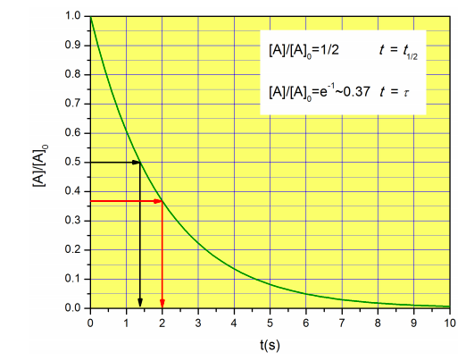
Note that in this case, the half-life does not depend on the initial concentration of A. This will not be the case for other types of mechanisms. Also, notice that we have already covered the concept of half-life in Chapter 1 (see Figure \(1.3.1\)), so this might be a good time to read that section again and refresh what we have already learned about sketching exponential decays.
In physical chemistry, scientists often talk about the ‘relaxation time’ instead of the half-life. The relaxation time \(\tau\) for a decay of the shape \(a^{-b t}\) is \(1/b\), so in this case, the relaxation time is simply \(1/k\). Notice that the relaxation time has units of time, and it represents the time at which the concentration has decayed to \(e^{-1}\) of its original value:
\[[A]=[A]_0e^{-t/\tau}\rightarrow \frac{[A]}{[A]_0}=e^{-t/\tau} \xrightarrow{t=\tau}\frac{[A]}{[A]_0}=e^{-1}\approx0.37 \nonumber\]
The half-life and relaxation time are compared in Figure \(\PageIndex{5}\) for a reaction with \(k=0.5 s^{-1}\).
Consecutive First Order Processes
We will now analyze a more complex mechanism, which involves the formation of an intermediate species (B):
\[A \overset{k_1}{\rightarrow}B\overset{k_2}{\rightarrow}C \nonumber\]
which is mathematically described by Equations \ref{cons1}, \ref{cons2} and \ref{cons3}. Let’s assume that initially the concentration of A is [A]\(_0\), and the concentrations of B and C are zero. In addition, we can write a mass balance, which for these initial conditions is expressed as:
\[[A](t)+[B](t)+[C](t)=[A]_0 \nonumber\]
Let’s summarize the equations we have:
\[\frac{d[A]}{dt}=-k_1[A]\label{consq1}\] \[\frac{d[B]}{dt}=k_1[A]-k_2[B]\label{consq2}\] \[\frac{d[C]}{dt}=k_2[B]\label{consq3}\] \[[A]+[B]+[C]=[A]_0\label{consq4}\] \[[A](t=0)=[A]_0\label{consq5}\] \[[B](t=0)=[C](t=0)=0\label{consq6}\]
Note that Equation \ref{consq4} is not independent from Equations \ref{consq1}-\ref{consq3}. If you take the derivative of \ref{consq4} you get \(d[A]/dt+d[B]/dt+d[C]/dt=0\), which is the same you get if you add Equations \ref{consq1}-\ref{consq3}. This means that Equations \ref{consq1}-\ref{consq4} are not all independent, and three of them are enough for us to solve the problem. As you will see, the mass balance (\ref{consq4}) will give us a very easy way of solving for [C] once we have [A] and [B], so we will use it instead of Equation \ref{consq3}.
We need to solve the system of Equations \ref{consq1}-\ref{consq6}, and although there are methods to solve systems of differential equations (e.g. using linear algebra), this one is easy enough that can be solved with what we learned so far. This is because not all equations contain all variables. In particular, Equation \ref{consq1} is a simple separable equation with dependent variable [A], which can be solved independently of [B] and [C]. We in fact just solved this equation in the First Order Reactions section, so let’s write down the result:
\[\label{eq:a(t)} [A](t)=[A]_0e^{-k_1t}\]
Equation \ref{consq2} contains two dependent variables, but luckily we just obtained an expression for one of them. We can now re-write \ref{consq2} as:
\[\label{consq7} \frac{d[B]}{dt}=k_1[A]_0e^{-k_1t}-k_2[B]\]
Equation \ref{consq7} contains only one dependent variable, [B], one independent variable, \(t\), and three constants: \(k_1\), \(k_2\) and \([A]_0\). This is therefore an ordinary differential equation, and if it is either separable or linear, we will be able to solve it with the techniques we learned in this chapter. Recall eq. [sep], and verify that Equation \ref{consq7} cannot be separated as
\[\frac{d[B]}{dt}=\frac{g([B])}{h(t)} \nonumber\]
Equation \ref{consq7} is not separable. Is it linear? Recall Equation \ref{linear} and check if you can write this equation as \(\frac{d[B]}{dt}+p(t) [B]=q(t)\). We in fact can:
\[\label{consq8} \frac{d[B]}{dt}+k_2[B]=k_1[A]_0e^{-k_1t}\]
Let’s use the list of steps delineated in Section 4.2. We need to calculate the integrating factor, \(e^{ \int p(x)dx }\), which in this case is \(e^{ \int k_2dt }=e^{k_2t}\). We then multiply Equation \ref{consq8} by the integrating factor:
\[\frac{d[B]}{dt}e^{k_2t}+k_2[B]e^{k_2t}=k_1[A]_0e^{-k_1t}e^{k_2t}=k_1[A]_0e^{(k_2-k_1)t} \nonumber\]
In the next step, we need to recognize that the left-hand side of the equation is the derivative of the product of the dependent variable times the integrating factor:
\[\frac{d}{dt}\left( [B]e^{k_2t}\right)=k_1[A]_0e^{(k_2-k_1)t} \nonumber\]
We then take ‘\(dt\)’ to the right side of the equation and integrate both sides:
\[\int d \left( [B]e^{k_2t}\right)=\int k_1[A]_0e^{(k_2-k_1)t}dt \nonumber\]
\[[B]e^{k_2t}=\frac{1}{k_2-k_1} k_1[A]_0e^{(k_2-k_1)t}+c \nonumber\]
\[[B]=\frac{1}{k_2-k_1} k_1[A]_0\frac{e^{(k_2-k_1)t}}{e^{k_2t}}+\frac{c}{e^{k_2t}} \nonumber\]
\[[B]=\frac{k_1}{k_2-k_1} [A]_0e^{-k_1t}+ce^{-k_2t} \nonumber\]
We have an arbitrary constant because this is a first order differential equation. Let’s calculate \(c\) using the initial condition \([B](t=0)=0\):
\[0=\frac{k_1}{k_2-k_1} [A]_0e^{-k_1 0}+ce^{-k_2 0}=\frac{k_1}{k_2-k_1} [A]_0+c \nonumber\]
\[c=-\frac{k_1}{k_2-k_1} [A]_0 \nonumber\]
And therefore,
\[[B]=\frac{k_1}{k_2-k_1} [A]_0e^{-k_1t}-\frac{k_1}{k_2-k_1} [A]_0e^{-k_2t} \nonumber\]
\[\label{eq:b(t)} [B]=\frac{k_1}{k_2-k_1} [A]_0\left(e^{-k_1t}-e^{-k_2t}\right)\]
Before moving on, notice that we have assumed that \(k_1\neq k_2\). We were not explicit, but we performed the integration with this assumption. If \(k_1=k_2\) the exponential term becomes 1, which is not a function of \(t\). In this case, the integral will obviously be different, so our answer assumes \(k_1\neq k_2\). This is good news, since otherwise we would need to worry about the denominator of [eq:b(t)] being zero. You will solve the case \(k_1= k_2\) in Problem 4.4.
Now that we have [A] and [B], we can get the expression for [C]. We could use Equation \ref{consq3}:
\[\frac{d[C]}{dt}=k_2[B]=\frac{k_2k_1}{k_2-k_1} [A]_0\left(e^{-k_1t}-e^{-k_2t}\right) \nonumber\]
This is not too difficult because the equation is separable. However, it is easier to get [C] from the mass balance, Equation \ref{consq4}:
\[[C]=[A]_0-[A]-[B] \nonumber\]
Plugging the answers we got for [A] and [B]:
\[[C]=[A]_0-[A]_0e^{-k_1t}-\frac{k_1}{k_2-k_1} [A]_0\left(e^{-k_1t}-e^{-k_2t}\right) \nonumber\]
\[\label{eq:c(t)} [C]=[A]_0\left[1-e^{-k_1t}-\frac{k_1}{k_2-k_1}\left(e^{-k_1t}-e^{-k_2t}\right)\right]\]
Equations \ref{eq:a(t)}, \ref{eq:b(t)}, \ref{eq:c(t)} are the solutions we were looking for. If we had the values of \(k_1\) and \(k_2\) we could plot \([A](t)/[A]_0\), \([B](t)/[A]_0\) and \([C](t)/[A]_0\) and see how the three species evolve with time. If we had \([A]_0\) we could plot the actual concentrations, but notice that this does not add too much, because it just re-scales the \(y-\)axis but does not change the shape of the curves.
Figure \(\PageIndex{6}\) shows the concentration profiles for a reaction with \(k_1=0.1 s^{-1}\) and \(k_2=0.5 s^{-1}\). Notice that because B is an intermediate, its concentration first increases, but then decreases as B is converted into C. The product C has a ‘lag phase’, because we need to wait until enough B is formed before we can see the concentration of C increase (first couple of seconds in this example). As you will see after solving your homework problems, the time at which the intermediate (B) achieves its maximum concentration depends on both \(k_1\) and \(k_2\).

Reversible first order reactions
So far we have discussed irreversible reactions. Yet, we know that many reactions are reversible, meaning that the reactant and product exist in equilibrium:
\[A \xrightleftharpoons[k_2]{k_1} B \nonumber\]
The rate of change of [A], \(\frac{d[A]}{dt}\), is the rate at which A appears (\(k_2[B]\)) minus the rate at which A disappears (\(k_1[A]\)):
\[\frac{d[A]}{dt}=k_2[B]-k_1[A] \nonumber\]
We cannot solve this equation as it is, because it has two dependent variables, [A] and [B]. However, we can write [B] in terms of [A], or [A] in terms of [B], by using the mass balance:
\[[A](t)+[B](t)=[A]_0+[B]_0 \nonumber\]
\[\frac{d[A]}{dt}=k_2\left( [A]_0+[B]_0-[A]\right)-k_1[A] \nonumber\]
\[\frac{d[A]}{dt}=k_2\left( [A]_0+[B]_0\right)-\left(k_2+k_1\right)[A] \nonumber\]
This is an ordinary, separable, first order differential equation, so it can be solved by direct integration. You will solve this problem in your homework, so let’s skip the steps and jump to the answer:
\[\label{eq:aeq} [A]=\frac{k_2\left ( [A]_0+[B]_0 \right )}{k_1+k_2}+\frac{k_1 [A]_0-k_2[B]_0 }{k_1+k_2}e^{-\left (k_1+k_2 \right )t}\]
This is a reversible reaction, so if we wait long enough it will reach equilibrium The concentration of [A] in equilibrium, [A]\(_{eq}\), is the limit of the previous expression when \(t\rightarrow \infty\). Because \(e^{-x}\rightarrow 0\) when \(x\rightarrow \infty\):
\[[A]_{eq}=\frac{k_2\left ( [A]_0+[B]_0 \right )}{k_1+k_2} \nonumber\]
and we can re-write Equation \ref{eq:aeq} as
\[\label{eq:aeq2} [A]=[A]_{eq}+\left([A]_0-[A]_{eq}\right)e^{-\left (k_1+k_2 \right )t}\]
As you will do in your homework, we can calculate \([B](t)\) from the mass balance as \([B](t)=[A]_0+[B]_0-[A](t)\).
Equation \ref{eq:aeq2} is not too different from Equation \ref{eq:mdecay}. In the case of an irreversible reaction, (Equation \ref{eq:mdecay}), [A] decays from an initial value [A]\(_0\) to a final value \([A]_{t \rightarrow \infty}=0\) with a relaxation time \(\tau=1/k\). For the reversible reaction, \([A]-[A]_{eq}\) decays from an initial value \([A]_0-[A]_{eq}\) to a final value \([A]_{t \rightarrow \infty}-[A]_{eq}=0\) with a relaxation time \(\tau=(k_1+k_2)^{-1}\). This last statement is not trivial! It says that the rate at which a reaction approaches equilibrium depends on the sum of the forward and backward rate constants.

In your homework you will be asked to prove that the ratio of the concentrations in equilibrium, \([B]_{eq}/[A]_{eq}\) is equal to the ratio of the forward and backwards rate constants. In addition, from your introductory chemistry courses you should know that the equilibrium constant of a reaction (\(K_{eq}\)) is the ratio of the equilibrium concentrations of product of reactant. Therefore:
\[\label{eq:eql} \frac{[B]_{eq}}{[A]_{eq}}=K_{eq}=\frac{k_1}{k_2}\]
This means that we can calculate the ratio of \(k_1\) and \(k_2\) from the concentrations of A and B we observe once equilibrium has been reached (i.e. once \(\frac{d[A]}{dt}=\frac{d[B]}{dt}=0\)). At the same time, we can obtain the sum of \(k_1\) and \(k_2\) from the relaxation time of the process. If we have the sum and the ratio, we can calculate both \(k_1\) and \(k_2\). This all makes sense, but it requires that we can watch the reaction from an initial state outside equilibrium. If the system is already in equilibrium, \([A]_0=[A]_{eq}\), and \(d[A]/dt=0\) at all times. A plot of [A]\((t)\) will look flat, and we will not be able to extract the relaxation time of the reaction. If, however, we have an experimental way of shifting the equilibrium so \([A]_0\neq[A]_{eq}\), we can measure the relaxation time by observing how the reaction returns to its equilibrium position.
Advanced topic: How can we shift the equilibrium? One way is to produce a very quick change in the temperature of the system. The equilibrium constant of a reaction usually depends on temperature, so if a system is equilibrated at a given temperature (say \(25^{\circ}C\)), and we suddenly increase the temperature (e.g. to \(26^{\circ}C\)), the reaction will suddenly be away from its equilibrium condition at the new temperature. We can watch the system relax to the equilibrium concentrations at \(26^{\circ}C\), and measure the relaxation time. This will allow us to calculate the rate constants at \(26^{\circ}C\).
\[\frac{[B]_{eq}}{[A]_{eq}}=K_{eq}=\frac{k_1}{k_2} \nonumber\]
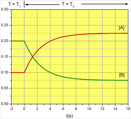
Advanced topic The following figure illustrates the experimental procedure known as “T-jump”, in which a sudden change in temperature is used to shift the position of a reversible reaction out of equilibrium. The experiment starts at a temperature \(T_1\), and the temperature is increased to \(T_2\) instantaneously at time \(t=0\). Because the equilibrium constant at \(T_2\) is different from the equilibrium constant at \(T_1\), the system needs to relax to the new equilibrium state. From the graph below estimate to the best of your abilities \(K_{eq} (T_1)\), \(K_{eq} (T_2)\), and the rate constants \(k_1\), and \(k_2\) at \(T_2\).
\[A \xrightleftharpoons[k_2]{k_1} B \nonumber\]
Solution
At \(T_1\), \([A]_{eq}=0.1 M\) and \([B]_{eq}=0.2 M\). The equilibrium constant is \([B]_{eq}/[A]_{eq}=2\).
At \(T_2\), \([A]_{eq}=0.225 M\) and \([B]_{eq}=0.075 M\). The equilibrium constant is \([B]_{eq}/[A]_{eq}=1/3\).
Because \(K_{eq}=\frac{k_1}{k_2}\), at \(T=T_2\), \(\frac{k_1}{k_2}=1/3\). To calculate the relaxation time let’s look at the expression for \([A](t)\) (Equation \ref{eq:aeq2}).
\[[A]=[A]_{eq}+\left([A]_0-[A]_{eq}\right)e^{-\left (k_1+k_2 \right )t} \nonumber\]
When the time equals the relaxation time (\(\tau=(k_1+k_2)^{-1}\)),
\[[A](t=\tau)=[A]_{eq}+\left([A]_0-[A]_{eq}\right)e^{-1} \nonumber\]
\[[A](t=\tau)\approx 0.225M+\left(0.1M-0.225M\right)\times 0.37\approx 0.18 \nonumber\]1
From the graph, \([A]=0.18\) at \(t = 2.5s\), and therefore the relaxation time is \(\tau=(k_1+k_2)^{-1}= 2.5s\).
We have \((k_1+k_2)^{-1}= 2.5s = 5/2 s\) and \(\frac{k_1}{k_2}=1/3\):
\[(k_1+k_2)=2/5= (k_1+3k_1)=4k_1\rightarrow k_1=1/10 = 0.1 s^{-1}, k_2=0.3 s^{-1} \nonumber\]