
3.1: Strategies for Geometry Optimization and Finding Transition States
- Page ID
- 11576

The extension of the harmonic and Morse vibrational models to polyatomic molecules requires that the multidimensional energy surface be analyzed in a manner that allows one to approximate the molecule’s motions in terms of many nearly independent vibrations. In this Section, we will explore the tools that one uses to carry out such an analysis of the surface, but first it is important to describe how one locates the minimum-energy and transition-state geometries on such surfaces.
Finding Local Minima
Many strategies that attempt to locate minima on molecular potential energy landscapes begin by approximating the potential energy \(V\) for geometries (collectively denoted in terms of \(3N\) Cartesian coordinates \(\{q_j\}\)) in a Taylor series expansion about some “starting point” geometry (i.e., the current molecular geometry in an iterative process or a geometry that you guessed as a reasonable one for the minimum or transition state that you are seeking):
\[V (g_k) = V(0) + \sum_k \left(\dfrac{\partial V}{\partial q_k}\right) q_k + \dfrac{1}{2} \sum_{j,k} q_j H_{j,k} q_k \, + \, ... \label{3.1.1}\]
Here,
- \(V(0)\) is the energy at the current geometry,
- \(\dfrac{\partial{V}}{\partial{q_k}} = g_k\) is the gradient of the energy along the \(q_k\) coordinate,
- \(H_{j,k} = \dfrac{\partial^2{V}}{\partial{q_j}\partial{q_k}}\) is the second-derivative or Hessian matrix, and
- \(g_k\) is the length of the “step” to be taken along this Cartesian direction.
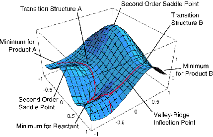
An example of an energy surface in only two dimensions is given in the Figure 3.1 where various special aspects are illustrated. For example, minima corresponding to stable molecular structures, transition states (first order saddle points) connecting such minima, and higher order saddle points are displayed.
If the only knowledge that is available is \(V(0)\) and the gradient components (e.g., computation of the second derivatives is usually much more computationally taxing than is evaluation of the gradient, so one is often forced to work without knowing the Hessian matrix elements), the linear approximation
\[V(q_k) = V(0) + \sum_k g_K \,q_k \label{3.1.2}\]
suggests that one should choose “step” elements \(q_k\) that are opposite in sign from that of the corresponding gradient elements \(g_k = \dfrac{\partial{V}}{\partial{q_k}}\) if one wishes to move “downhill” toward a minimum. The magnitude of the step elements is usually kept small in order to remain within the “trust radius” within which the linear approximation to \(V\) is valid to some predetermined desired precision (i.e., one wants to assure that \(\sum_k g_K q_k\) is not too large).
When second derivative data is available, there are different approaches to predicting what step {\(g_k\)} to take in search of a minimum, and it is within such Hessian-based strategies that the concept of stepping along \(3N-6\) independent modes arises. We first write the quadratic Taylor expansion
\[V (g_k) = V(0) + \sum_k g_K g_k + \dfrac{1}{2} \sum_{j,k} q_j H_{j,k} g_k\label{3.1.3}\]
in matrix-vector notation
\[V(\textbf{q}) = V(0) + \textbf{q}^{\textbf{T}} \cdot \textbf{g} + \dfrac{1}{2} \textbf{q}^{\textbf{T}} \cdot \textbf{H} \cdot \textbf{q} \label{3.1.4}\]
with the elements \(\{g_k\}\) collected into the column vector \(\textbf{q}\) whose transpose is denoted \(\textbf{q}^{\textbf{T}}\).
Introducing the unitary matrix \(\textbf{U}\) that diagonalizes the symmetric \(\textbf{H}\) matrix, the above equation becomes
\[V(\textbf{q}) = V(0) + \textbf{q}^{\textbf{T}} \textbf{U} \, \textbf{U}^{\textbf{T}} \textbf{q} + \dfrac{1}{2} \textbf{q}^{\textbf{T}} \textbf{U} \, \textbf{U}^{\textbf{T}} \textbf{H} \textbf{U}\, \textbf{U}^{\textbf{T}} \textbf{q}. \label{3.1.5}\]
Because \(\textbf{U}^{\textbf{T}}\textbf{H}\textbf{U}\) is diagonal, we have
\[(\textbf{U}^{\textbf{T}}\textbf{H}\textbf{U})_{k,l} = \delta_{k,l} \lambda_k \label{3.1.6}\]
where \(\lambda_k\) are the eigenvalues of the Hessian matrix. For non-linear molecules, \(3N-6\) of these eigenvalues will be non-zero; for linear molecules, \(3N-5\) will be non-zero. The 5 or 6 zero eigenvalues of \(\textbf{H}\) have eigenvectors that describe translation and rotation of the entire molecule; they are zero because the energy surface \(V\) does not change if the molecule is rotated or translated. It can be difficult to properly identify the 5 or 6 translation and rotation eigenvalues of the Hessian because numerical precision issues often cause them to occur as very small positive or negative eigenvalues. If the molecule being studied actually does possess internal (i.e., vibrational) eigenvalues that are very small (e.g., the torsional motion of the methyl group in ethane has a very small energy barrier as a result of which the energy is very weakly dependent on this coordinate), one has to be careful to properly identify the translation-rotation and internal eigenvalues. By examining the eigenvectors corresponding to all of the low Hessian eigenvalues, one can identify and thus separate the former from the latter. In the remainder of this discussion, I will assume that the rotations and translations have been properly identified and the strategies I discuss will refer to utilizing the remaining \(3N-5\) or \(3N-6\) eigenvalues and eigenvectors to carry out a series of geometry “steps” designed to locate energy minima and transition states.
The eigenvectors of \(\textbf{H}\) form the columns of the array \(U\) that brings \(H\) to diagonal form:
\[\sum_{\lambda} H_{k,l} U_{l,m} = \lambda_m U_{k,m} \label{3.1.7}\]
Therefore, if we define
\[Q_m = \sum_k U^T_{m,k} g_k \label{3.1.8a}\]
and
\[G_m = \sum_k U^T_{m,k} g_K \label{3.1.8b}\]
to be the component of the step \(\{g_k\}\) and of the gradient along the \(m^{th}\) eigenvector of \(H\), the quadratic expansion of \(V\) can be written in terms of steps along the \(3N-5\) or \(3N-6 \{Q_m\}\) directions that correspond to non-zero Hessian eigenvalues:
\[V (g_k) = V(0) + \sum_m G^T_m Q_m + \dfrac{1}{2} \sum_m Q_m \lambda_m Q_m.\label{3.1.9}\]
The advantage to transforming the gradient, step, and Hessian to the eigenmode basis is that each such mode (labeled m) appears in an independent uncoupled form in the expansion of \(V\). This allows us to take steps along each of the \(Q_m\) directions in an independent manner with each step designed to lower the potential energy when we are searching for minima (strategies for finding a transition state will be discussed below).
For each eigenmode direction, one can ask for what size step \(Q\) would the quantity \(GQ + \dfrac{1}{2} \lambda Q^2\) be a minimum. Differentiating this quadratic form with respect to \(Q\) and setting the result equal to zero gives
\[Q_m = - \dfrac{G_m}{\lambda_m} \label{3.1.10}\]
that is, one should take a step opposite the gradient but with a magnitude given by the gradient divided by the eigenvalue of the Hessian matrix. If the current molecular geometry is one that has all positive \(\lambda_m\) values, this indicates that one may be “close” to a minimum on the energy surface (because all \(\lambda_m\) are positive at minima). In such a case, the step \(Q_m = - G_m/\lambda_m\) is opposed to the gradient along all \(3N-5\) or \(3N-6\) directions, much like the gradient-based strategy discussed earlier suggested. The energy change that is expected to occur if the step \(\{Q_m\}\) is taken can be computed by substituting \(Q_m = - G_m/\lambda_m\) into the quadratic equation for \(V\):
\[V(\text{after step}) = V(0) + \sum_m G^T_m \bigg(- \dfrac{G_m}{\lambda_m}\bigg) + \dfrac{1}{2} \sum_m \lambda_m \bigg(- \dfrac{G_m}{\lambda_m}\bigg)^2 \label{3.1.11a}\]
\[= V(0) - \dfrac{1}{2} \sum_m \lambda_m \bigg(- \dfrac{G_m}{\lambda_m}\bigg)^2. \label{3.1.11b}\]
This clearly suggests that the step will lead “downhill” in energy along each eigenmode as long as all of the \(\lambda_m\) values are positive. For example, if one were to begin with a good estimate for the equilibrium geometries of ethylene and propene, one could place these two molecules at a distance \(R_0\) longer than the expected inter-fragment equilibrium distance \(R_{\rm vdW}\) in the van der Waals complex formed when they interact. Because both fragments are near their own equilibrium geometries and at a distance \(R_0\) at which long-range attractive forces will act to draw them together, a strategy such as outlined above could be employed to locate the van der Waals minimum on their energy surface. This minimum is depicted qualitatively in Figure 3.1a.

Beginning at \(R_0\), one would find that \(3N-6 = 39\) of the eigenvalues of the Hessian matrix are non-zero, where \(N = 15\) is the total number of atoms in the ethylene-propene complex. Of these 39 non-zero eigenvalues, three will have eigenvectors describing radial and angular displacements of the two fragments relative to one another; the remaining 36 will describe internal vibrations of the complex. The eigenvalues belonging to the inter-fragment radial and angular displacements may be positive or negative (because you made no special attempt to orient the molecules at optimal angles and you may not have guessed very well at optimal the equilibrium inter-fragment distance), so it would probably be wisest to begin the energy-minimization process by using gradient information to step downhill in energy until one reaches a geometry \(R_1\) at which all 39 of the Hessian matrix eigenvalues are positive. From that point on, steps determined by both the gradient and Hessian (i.e., \(Q_m = - G_m/\lambda_m\)) can be used unless one encounters a geometry at which one of the eigenvalues \(\lambda_m\) is very small, in which case the step \(Q_m = - G_m/\lambda_m\) along this eigenmode could be unrealistically large. In this case, it would be better to not take \(Q_m = - G_m/\lambda_m\) for the step along this particular direction but to take a small step in the direction opposite to the gradient to improve chances of moving downhill. Such small-eigenvalue issues could arise, for example, if the torsion angle of propene’s methyl group happened, during the sequence of geometry steps, to move into a region where eclipsed rather than staggered geometries are accessed. Near eclipsed geometries, the Hessian eigenvalue describing twisting of the methyl group is negative; near staggered geometries, it is positive.
Whenever one or more of the \(\lambda_m\) are negative at the current geometry, one is in a region of the energy surface that is not sufficiently close to a minimum to blindly follow the prescription \(Q_m = - G_m/\lambda_m\) along all modes. If only one \(\lambda_m\) is negative, one anticipates being near a transition state (at which all gradient components vanish and all but one \(\lambda_m\) are positive with one \(\lambda_m\) negative). In such a case, the above analysis suggests taking a step \(Q_m = - G_m/\lambda_m\) along all of the modes having positive \(\lambda_m\), but taking a step of opposite direction (e.g., \(Q_n = - G_n/\lambda_n\) unless \(\lambda_m\) is very small in which case a small step opposite \(G_n\) is best) along the direction having negative \(\lambda_n\) if one is attempting to move toward a minimum. This is what I recommended in the preceding paragraph when an eclipsed geometry (which is a transition state for rotation of the methyl group) is encountered if one is seeking an energy minimum.
Finding Transition States
On the other hand, if one is in a region where one Hessian eigenvalues is negative (and the rest are positive) and if one is seeking to find a transition state, then taking steps \(Q_m = - G_m/\lambda_m\) along all of the modes Having positive eigenvalues and taking \(Q_n = - G_n/\lambda_n\) along the mode having negative eigenvalue is appropriate. The steps \(Q_m = - G_m/\lambda_m\) will act to keep the energy near its minimum along all but one direction, and the step \(Q_n = - G_n/\lambda_n\) will move the system uphill in energy along the direction having negative curvature, exactly as one desires when “walking” uphill in a streambed toward a mountain pass.
However, even the procedure just outlined for finding a transition state can produce misleading results unless some extent of chemical intuition is used. Let me give an example to illustrate this point. Let’s assume that one wants to find begin near the geometry of the van der Waals complex involving ethylene and propene and to then locate the transition state on the reaction path leading to the [2+2] cyclo-addition products methyl-cyclobutane as also shown in Figure 3.1a. Consider employing either of two strategies to begin the “walk” leading from the van der Waals complex to the desired transition state (TS):
- One could find the lowest (non-translation or non-rotation) Hessian eigenvalue and take a small step uphill along this direction to begin a streambed walk that might lead to the TS. Using the smallest Hessian eigenvalue to identify a direction to explore makes sense because it is along this direction that the energy surface rises least abruptly (at least near the geometry of the reactants).
- One could move the ethylene radially a bit (say 0.2 Å) closer to the propene to generate an initial geometry to begin the TS search. This makes sense because one knows the reaction must lead to inter-fragment carbon-carbon distances that are much shorter in the methyl-cyclobutane products than in the van der Waals complex.
The first strategy suggested above will likely fail because the series of steps generated by walking uphill along the lowest Hessian eigenmode will produce a path leading from eclipsed to staggered orientation of propene’s methyl group. Indeed, this path leads to a TS, but it is not the [2+2] cyclo-addition TS that we want. The take-home lesson here is that uphill streambed walks beginning at a minimum on the reactants’ potential energy surface may or may not lead to the desired TS. Such walks are not foolish to attempt, but one should examine the nature of the eigenmode being followed to judge whether displacements along this mode make chemical sense. Clearly, only rotating the methyl group is not a good way to move from ethylene and propene to methyl-cyclobutane.
The second strategy suggested above might succeed, but it would probably still need to be refined. For example, if the displacement of the ethylene toward the propene were too small, one would not have distorted the system enough to move it into a region where the energy surface has negative curvature along the reaction path as it must have as one approaches the TS. So, if the Hessian eigenmodes whose eigenvectors possess substantial inter-fragment radial displacements are all positive, one has probably not moved the two fragments close enough together. Probably the best way to then proceed would be to move the two fragments even closer (or, to move them along a linear synchronous path[1] connecting the reactants and products) until one finds a geometry at which a negative Hessian eigenvalue’s eigenmode has substantial components along what appears to be reasonable for the desired reaction path (i.e., substantial displacements leading to shorter inter-fragment carbon-carbon distances). Once one has found such a geometry, one can use the strategies detailed earlier (e.g., \(Q_m = - G_m/\lambda_m\) to then walk uphill along one mode while minimizing along the other modes to move toward the TS. If successful, such a process will lead to the TS at which all components of the gradient vanish and all but one eigenvalue of the Hessian is positive. The take-home lesson of the example is it is wise to try to first find a geometry close enough to the TS to cause the Hessian to have a negative eigenvalue whose eigenvector has substantial character along directions that make chemical sense for the reaction path.
In either a series of steps toward a minimum or toward a TS, once a step has been suggested within the eigenmode basis, one needs to express that step in terms of the original Cartesian coordinates \(q_k\) so that these Cartesian values can be altered within the software program to effect the predicted step. Given values for the \(3N-5\) or \(3N-6\) step components \(Q_m\) (n.b., the step components \(Q_m\) along the 5 or 6 modes having zero Hessian eigenvalues can be taken to be zero because the would simply translate or rotate the molecule), one must compute the {\(g_k\)}. To do so, we use the relationship
\[Q_m = \sum_k U^T_{m,k} g_k\label{3.1.12}\]
and write its inverse (using the unitary nature of the \(\textbf{U}\) matrix):
\[g_k = \sum_m U_{k,m} Q_m \label{3.1.13}\]
to compute the desired Cartesian step components.
In using the Hessian-based approaches outlined above, one has to take special care when one or more of the Hessian eigenvalues is small. This often happens when
- one has a molecule containing “soft modes” (i.e., degrees of freedom along which the energy varies little), or
- as one moves from a region of negative curvature into a region of positive curvature (or vice versa)- in such cases, the curvature must move through or near zero.
For these situations, the expression \(Q_m = - G_m/\lambda_m\) can produce a very large step along the mode having small curvature. Care must be taken to not allow such incorrect artificially large steps to be taken.
Energy Surface Intersections
I should note that there are other important regions of potential energy surfaces that one must be able to locate and characterize. Above, we focused on local minima and transition states. Later in this Chapter, and again in Chapter 8, we will discuss how to follow so-called reaction paths that connect these two kinds of stationary points using the type of gradient and Hessian information that we introduced earlier in this Chapter.
It is sometimes important to find geometries at which two Born-Oppenheimer energy surfaces \(V_1(\text{q})\) and \(V_2(\text{q})\) intersect because such regions often serve as efficient funnels for trajectories or wave packets evolving on one surface to undergo so-called non-adiabatic transitions to the other surface. Let’s spend a few minutes thinking about under what circumstances such surfaces can indeed intersect, because students often hear that surfaces do not intersect but, instead, undergo avoided crossings. To understand the issue, let us assume that we have two wave functions \(\Phi_1\) and \(\Phi_2\) both of which depend on \(3N-6\) coordinates \(\{q\}\). These two functions are not assumed to be exact eigenfunctions of the Hamiltonian \(H\), but likely are chosen to approximate such eigenfunctions. To find the improved functions \(\Psi_1\) and \(\Psi_2\) that more accurately represent the eigenstates, one usually forms linear combinations of \(\Phi_1\) and \(\Phi_2\),
\[ \Psi_K = C_{K,1} \Phi_1 + C_{K,2} \Phi_2 \label{3.1.14}\]
from which a 2x2 matrix eigenvalue problem arises:
\[\left|\begin{array}{cc}
H_{1,1}-E & H_{1,2}\\
H_{2,1} & H_{2,2}-E
\end{array}\right|=0\]
This quadratic equation has two solutions
\[ 2E_\mp = (H_{1,1} + H_{2,2}) \pm \sqrt{(H_{1,1}+H_{2,2})^2 + 4H_{1,2}^2}\]
These two solutions can be equal (i.e., the two state energies can cross) only if the square root factor vanishes. Because this factor is a sum of two squares (each thus being positive quantities), this can only happen if two identities hold simultaneously (i.e., at the same geometry):
\[H_{1,1} = H_{2,2} \label{3.1.15a}\]
and
\[H_{1,2} = 0. \label{3.1.15b}\]
The main point then is that in the \(3N-6\) dimensional space, the two states will generally not have equal energy. However, in a space of two lower dimensions (because there are two conditions that must simultaneously be obeyed: \(H_{1,1} = H_{2,2}\) and \(H_{1,2} = 0\)), their energies may be equal. They do not have to be equal, but it is possible that they are. It is based upon such an analysis that one usually says that potential energy surfaces in \(3N-6\) dimensions may undergo intersections in spaces of dimension \(3N-8\). If the two states are of different symmetry (e.g., one is a singlet and the other a triplet), the off-diagonal element \(H_{1,2}\) vanishes automatically, so only one other condition is needed to realize crossing. So, we say that two states of different symmetry can cross in a space of dimension \(3N-7\). For a triatomic molecule with \(3N-6 = 3\) internal degrees of freedom, this means that surfaces of the same symmetry can cross in a space of dimension 1 (i.e., along a line) while those of different symmetry can cross in a space of dimension 2 (i.e., in a plane). An example of such a surface intersection is shown in Figure 3.1c.
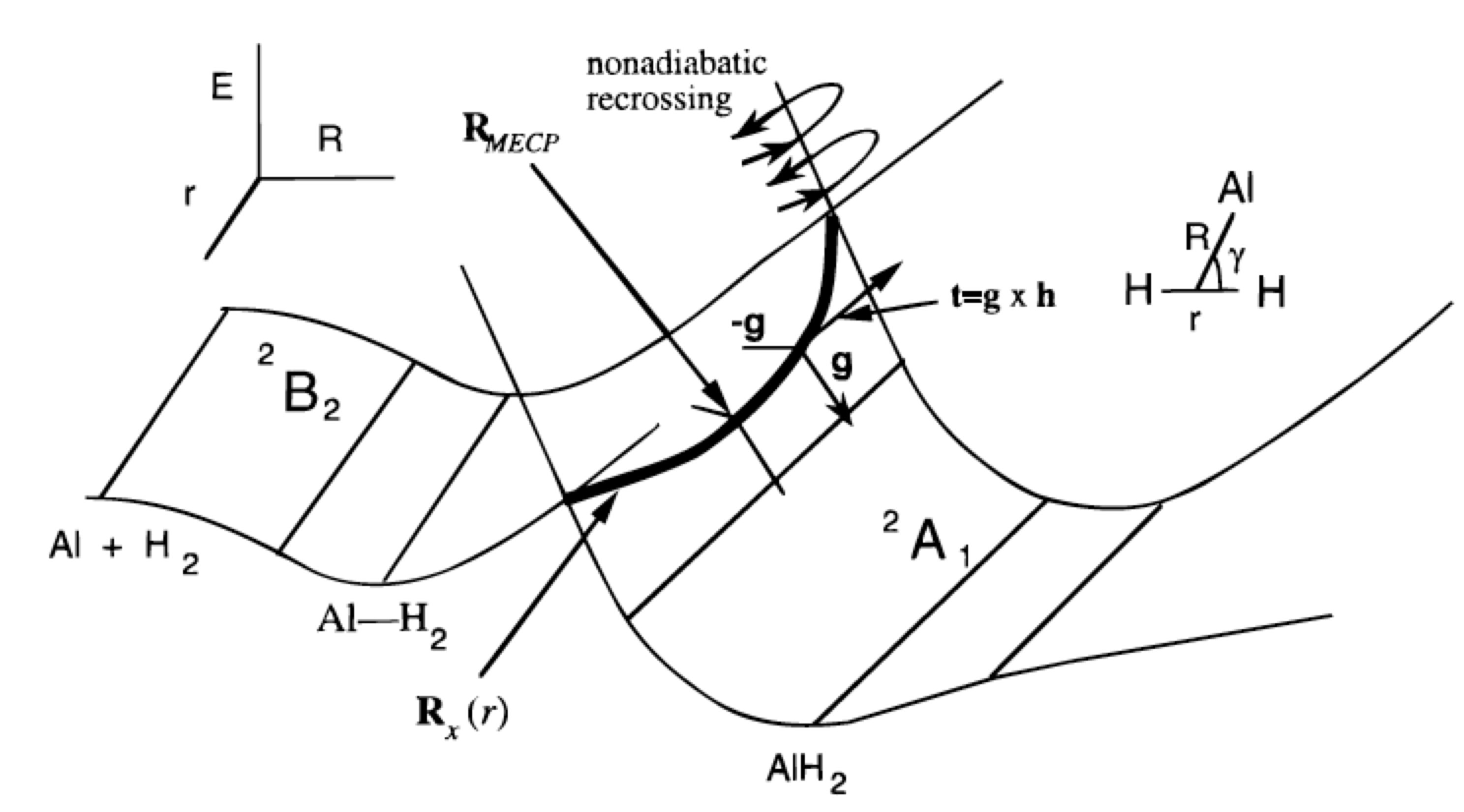
First considering the reaction of Al (3s2 3p1; 2P) with \(H_2 (sg2; 1Sg+)\) to form AlH2(^^2A_1) as if it were to occur in \(C_{2v}\) symmetry, the \(Al\) atom’s occupied 3p orbital can be directed in either of three ways.
- If it is directed toward the midpoint of the H-H bond, it produces an electronic state of \(^2A_1\) symmetry.
- If it is directed out of the plane of the \(AlH_2\), it gives a state of \(2B_1\) symmetry, and
- if it is directed parallel to the H-H bond, it generates a state of \(^2B_2\) symmetry.
The \(^2A_1\) state is, as shown in the upper left of Figure 3.1c, repulsive as the Al atom’s 3s and 3p orbitals begin to overlap with the hydrogen molecule’s \(\sigma_g\) orbital at large \(R\)-values. The \(^2B_2\) state, in which the occupied 3p orbital is directed sideways parallel to the H-H bond, leads to a shallow van der Waals well at long-R but also moves to higher energy at shorter \(R\)-values.
The ground state of the \(AlH_2\) molecule has its five valence orbitals occupied as follows:
- two electrons occupy a bonding Al-H orbital of \(a_1\) symmetry,
- two electrons occupy a bonding Al-H orbital of \(b_2\) symmetry, and
- the remaining electron occupies a non-bonding orbital of \(sp^2\) character localized on the Al atom and having a1 symmetry.
This \(a_1^2 b_2^2 a_1^1\) orbital occupancy of the \(AlH_2\) molecule’s ground state does not correlate directly with any of the three degenerate configurations of the ground state of \(Al + H_2\) which are \(a_1^2 a_1^2 a_1^1, a_1^2 a_1^2 b_1^1\), and \(a_1^2 a_1^2 b_2^1\) as explained earlier. It is this lack of direct configuration correlation that generates the reaction barrier show in Figure 3.1c.
Let us now return to the issue of finding the lower-dimensional (\(3N-8\) or \(3N-7\)) space in which two surfaces cross, assuming one has available information about the gradients and Hessians of both of these energy surfaces \(V_1\) and \(V_2\). There are two components of characterizing the intersection space within which \(V_1\) = \(V_2\):
- One has to first locate one geometry \(\textbf{q}_0\) lying within this space and then,
- one has to sample nearby geometries (e.g., that might have lower total energy) lying within this subspace where \(V_1 = V_2\).
To locate a geometry at which the difference function \(F = [V_1 –V_2]^2\) passes through zero, one can employ conventional functional minimization methods, such as those detailed earlier when discussing how to find energy minima, to locate where \(F = 0\), but now the function one is seeking to locate a minimum on is the potential energy surface difference.
Once one such geometry \(\textbf{q}_0\) has been located, one subsequently tries to follow the seam (i.e., for a triatomic molecule, this is the one-dimensional line of crossing; for larger molecules, it is a \(3N-8\) dimensional space) within which the function \(F\) remains zero. Professor David Yarkony has developed efficient routines for characterizing such subspaces (D. R. Yarkony, Acc. Chem. Res. 31, 511-518 (1998)). The basic idea is to parameterize steps away from (\(q_0\)) in a manner that constrains such steps to have no component along either the gradient of (\(H_{1,1} –H_{2,2}\)) or along the gradient of \(H_{1,2}\). Because \(V_1 = V_2\) requires having both \(H_{1,1} = H_{2,2}\) and \(H_{1,2} = 0\), taking steps obeying these two constraints allows one to remain within the subspace where \(H_{1,1} = H_{2,2}\) and \(H_{1,2} = 0\) are simultaneously obeyed. Of course, it is a formidable task to map out the entire \(3N-8\) or \(3N-7\) dimensional space within which the two surfaces intersect, and this is essentially never done. Instead, it is common to try to find, for example, the point within this subspace at which the two surfaces have their lowest energy. An example of such a point is labeled RMECP in Figure 3.1c, and would be of special interest when studying reactions taking place on the lower-energy surface that have to access the surface-crossing seam to evolve onto the upper surface. The energy at RMECP reflects the lowest energy needed to access this surface crossing.
Such intersection seam location procedures are becoming more commonly employed, but are still under very active development, so I will refer the reader to Prof. Yarkony’s paper cited above for further guidance. For now, it should suffice to say that locating such surface intersections is an important ingredient when one is interested in studying, for example, photochemical reactions in which the reactants and products may move from one electronic surface to another, or thermal reactions that require the system to evolve onto an excited state through a surface crossing.
Endnotes
- This is a series of geometries \(R_x\) defined through a linear interpolation (using a parameter \(0 < x < 1\)) between the \(3N\) Cartesian coordinates \(R_{\rm reactants}\) belonging to the equilibrium geometry of the reactants and the corresponding coordinates \(R_{\rm products}\) of the products: \(R_x = R_{\rm reactants} x + (1-x) R_{\rm products}\)
Contributors and Attributions
Jack Simons (Henry Eyring Scientist and Professor of Chemistry, U. Utah) Telluride Schools on Theoretical Chemistry
Integrated by Tomoyuki Hayashi (UC Davis)