4.4: Preservation of Phase Space Volume and Liouville's Theorem
- Page ID
- 5104
\( \newcommand{\vecs}[1]{\overset { \scriptstyle \rightharpoonup} {\mathbf{#1}} } \)
\( \newcommand{\vecd}[1]{\overset{-\!-\!\rightharpoonup}{\vphantom{a}\smash {#1}}} \)
\( \newcommand{\id}{\mathrm{id}}\) \( \newcommand{\Span}{\mathrm{span}}\)
( \newcommand{\kernel}{\mathrm{null}\,}\) \( \newcommand{\range}{\mathrm{range}\,}\)
\( \newcommand{\RealPart}{\mathrm{Re}}\) \( \newcommand{\ImaginaryPart}{\mathrm{Im}}\)
\( \newcommand{\Argument}{\mathrm{Arg}}\) \( \newcommand{\norm}[1]{\| #1 \|}\)
\( \newcommand{\inner}[2]{\langle #1, #2 \rangle}\)
\( \newcommand{\Span}{\mathrm{span}}\)
\( \newcommand{\id}{\mathrm{id}}\)
\( \newcommand{\Span}{\mathrm{span}}\)
\( \newcommand{\kernel}{\mathrm{null}\,}\)
\( \newcommand{\range}{\mathrm{range}\,}\)
\( \newcommand{\RealPart}{\mathrm{Re}}\)
\( \newcommand{\ImaginaryPart}{\mathrm{Im}}\)
\( \newcommand{\Argument}{\mathrm{Arg}}\)
\( \newcommand{\norm}[1]{\| #1 \|}\)
\( \newcommand{\inner}[2]{\langle #1, #2 \rangle}\)
\( \newcommand{\Span}{\mathrm{span}}\) \( \newcommand{\AA}{\unicode[.8,0]{x212B}}\)
\( \newcommand{\vectorA}[1]{\vec{#1}} % arrow\)
\( \newcommand{\vectorAt}[1]{\vec{\text{#1}}} % arrow\)
\( \newcommand{\vectorB}[1]{\overset { \scriptstyle \rightharpoonup} {\mathbf{#1}} } \)
\( \newcommand{\vectorC}[1]{\textbf{#1}} \)
\( \newcommand{\vectorD}[1]{\overrightarrow{#1}} \)
\( \newcommand{\vectorDt}[1]{\overrightarrow{\text{#1}}} \)
\( \newcommand{\vectE}[1]{\overset{-\!-\!\rightharpoonup}{\vphantom{a}\smash{\mathbf {#1}}}} \)
\( \newcommand{\vecs}[1]{\overset { \scriptstyle \rightharpoonup} {\mathbf{#1}} } \)
\( \newcommand{\vecd}[1]{\overset{-\!-\!\rightharpoonup}{\vphantom{a}\smash {#1}}} \)
\(\newcommand{\avec}{\mathbf a}\) \(\newcommand{\bvec}{\mathbf b}\) \(\newcommand{\cvec}{\mathbf c}\) \(\newcommand{\dvec}{\mathbf d}\) \(\newcommand{\dtil}{\widetilde{\mathbf d}}\) \(\newcommand{\evec}{\mathbf e}\) \(\newcommand{\fvec}{\mathbf f}\) \(\newcommand{\nvec}{\mathbf n}\) \(\newcommand{\pvec}{\mathbf p}\) \(\newcommand{\qvec}{\mathbf q}\) \(\newcommand{\svec}{\mathbf s}\) \(\newcommand{\tvec}{\mathbf t}\) \(\newcommand{\uvec}{\mathbf u}\) \(\newcommand{\vvec}{\mathbf v}\) \(\newcommand{\wvec}{\mathbf w}\) \(\newcommand{\xvec}{\mathbf x}\) \(\newcommand{\yvec}{\mathbf y}\) \(\newcommand{\zvec}{\mathbf z}\) \(\newcommand{\rvec}{\mathbf r}\) \(\newcommand{\mvec}{\mathbf m}\) \(\newcommand{\zerovec}{\mathbf 0}\) \(\newcommand{\onevec}{\mathbf 1}\) \(\newcommand{\real}{\mathbb R}\) \(\newcommand{\twovec}[2]{\left[\begin{array}{r}#1 \\ #2 \end{array}\right]}\) \(\newcommand{\ctwovec}[2]{\left[\begin{array}{c}#1 \\ #2 \end{array}\right]}\) \(\newcommand{\threevec}[3]{\left[\begin{array}{r}#1 \\ #2 \\ #3 \end{array}\right]}\) \(\newcommand{\cthreevec}[3]{\left[\begin{array}{c}#1 \\ #2 \\ #3 \end{array}\right]}\) \(\newcommand{\fourvec}[4]{\left[\begin{array}{r}#1 \\ #2 \\ #3 \\ #4 \end{array}\right]}\) \(\newcommand{\cfourvec}[4]{\left[\begin{array}{c}#1 \\ #2 \\ #3 \\ #4 \end{array}\right]}\) \(\newcommand{\fivevec}[5]{\left[\begin{array}{r}#1 \\ #2 \\ #3 \\ #4 \\ #5 \\ \end{array}\right]}\) \(\newcommand{\cfivevec}[5]{\left[\begin{array}{c}#1 \\ #2 \\ #3 \\ #4 \\ #5 \\ \end{array}\right]}\) \(\newcommand{\mattwo}[4]{\left[\begin{array}{rr}#1 \amp #2 \\ #3 \amp #4 \\ \end{array}\right]}\) \(\newcommand{\laspan}[1]{\text{Span}\{#1\}}\) \(\newcommand{\bcal}{\cal B}\) \(\newcommand{\ccal}{\cal C}\) \(\newcommand{\scal}{\cal S}\) \(\newcommand{\wcal}{\cal W}\) \(\newcommand{\ecal}{\cal E}\) \(\newcommand{\coords}[2]{\left\{#1\right\}_{#2}}\) \(\newcommand{\gray}[1]{\color{gray}{#1}}\) \(\newcommand{\lgray}[1]{\color{lightgray}{#1}}\) \(\newcommand{\rank}{\operatorname{rank}}\) \(\newcommand{\row}{\text{Row}}\) \(\newcommand{\col}{\text{Col}}\) \(\renewcommand{\row}{\text{Row}}\) \(\newcommand{\nul}{\text{Nul}}\) \(\newcommand{\var}{\text{Var}}\) \(\newcommand{\corr}{\text{corr}}\) \(\newcommand{\len}[1]{\left|#1\right|}\) \(\newcommand{\bbar}{\overline{\bvec}}\) \(\newcommand{\bhat}{\widehat{\bvec}}\) \(\newcommand{\bperp}{\bvec^\perp}\) \(\newcommand{\xhat}{\widehat{\xvec}}\) \(\newcommand{\vhat}{\widehat{\vvec}}\) \(\newcommand{\uhat}{\widehat{\uvec}}\) \(\newcommand{\what}{\widehat{\wvec}}\) \(\newcommand{\Sighat}{\widehat{\Sigma}}\) \(\newcommand{\lt}{<}\) \(\newcommand{\gt}{>}\) \(\newcommand{\amp}{&}\) \(\definecolor{fillinmathshade}{gray}{0.9}\)Consider a phase space volume element \(dx_0\) at t=0, containing a small collection of initial conditions on a set of trajectories. The trajectories evolve in time according to Hamilton's equations of motion, and at a time t later will be located in a new volume element \(dx_t\) as shown in the figure below:
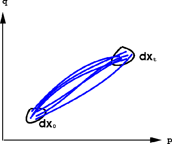
How is \(dx_0\) related to \(dx_t\)dxdd ? To answer this, consider a trajectory starting from a phase space vector \(x_0\) in \(dx_0\) and having a phase space vector \(x_t\) at time \(t\) in \(dx_t\). Since the solution of Hamilton's equations depends on the choice of initial conditions, \(x_t\) depends on \(x_0\) :
\[ \begin{align*} x_0 &= \left ( p_1 (0), \cdots , p_N(0), r_1(0), \cdots , r_N (0) \right ) \\[4pt] x_0 &= \left ( p_1 (t), \cdots , p_N(t), r_1(t), \cdots , r_N (t) \right ) \\[4pt] x^i_t &= x^i_t \left ( x^1_0 , \cdots , x^{6N}_0 \right ) \end{align*} \]
Thus, the phase space vector components can be viewed as a coordinate transformation on the phase space from \(t=0\) to time \(t\). The phase space volume element then transforms according to
\[ dx_t = J (x_t ; x_0 ) dx_0 \nonumber \]
where \(J (x_t ; x_0 )\) is the Jacobian of the transformation:
\[ J (x_t ; x_0 ) = \frac {\partial (x^1_t \cdots x^n_t )}{\partial (x^1_0 \cdots x^n_0 )} \nonumber \]
where \(n=6N\). The precise form of the Jacobian can be determined as will be demonstrated below.
The Jacobian is the determinant of a matrix \(M\),
\[ J (x_t ; x_0 ) = \text {det} (M) = e^{TrlnM} \nonumber \]
whose matrix elements are
\[ M_{ij} = \frac {\partial x^i_t}{\partial x^j_0} \nonumber \]
Taking the time derivative of the Jacobian, we therefore have
\[ \frac {dJ}{dt} = Tr \left ( M^{-1} \frac {dM}{dt} \right ) e^{TrlnM} \nonumber \]
\[ = J \sum _{i=1}^n \sum _{j=1}^n M^{-1}_{ij} \frac {dM_{ij}}{dt} \nonumber \]
The matrices \(M_{-1} \) and \( \frac {dM}{dt} \) can be seen to be given by
\[ M^{-1}_{ij} = \frac {\partial x^i_0}{\partial x^j_t} \nonumber \]
\[\frac {dM_{ji}}{dt} = \frac {\partial \dot {x}^i_t}{\partial x^i_0} \nonumber \]
Substituting into the expression for \(dJ/dt\) gives
\[\begin{align*} \frac {dJ}{dt} &= J \sum _{i,j=1}^n \frac {\partial x^i_0}{\partial x^j_t} \frac {\partial \dot {x}^i_t}{\partial x^i_0} \\[4pt] &= J \sum _{i,j,k=1}^n \frac {\partial x^i_0}{\partial x^j_t} \frac {\partial \dot {x}^i_t}{\partial x^k_t} \frac {\partial x^k_t}{\partial x^i_0} \end{align*} \]
where the chain rule has been introduced for the derivative \(\frac {\partial x^j_t}{\partial x^i_0}\). The sum over i can now be performed:
\[\sum _{i=1}^n \frac {\partial x^i_0}{\partial x^j_t} \frac {\partial x^k_t}{\partial x^i_0} = \sum ^n_{i=1} M^{-1}_{ij} M_{ki} = \sum ^n_{i=1} M_{ki}M^{-1}_{ij} = \delta _{kj} \nonumber \]
Thus,
\[\frac {dJ}{dt} = J \sum ^n_{j,k=1} \delta _{jk} \frac {\partial \dot {x}^j_t}{\partial x^k_0} \nonumber \]
\[ J \sum ^n_{j=1} \frac {\partial \dot {x}^j_t}{\partial x^j_t} = J \nabla _x \cdot \dot {x} \nonumber \]
or
\[ \frac {dJ}{dt} = J \nabla _x \cdot \dot {x} \nonumber \]
The initial condition on this differential equation is \(J (0) \equiv J (x_0; x_0) = 1 \). Moreover, for a Hamiltonian system \(\nabla _x \cdot \dot {x} = 0 \). This says that \(dJ/dt=0\) and \(J(0)=1\). Thus, \(J (x_t ; x_0 ) = 1 \). If this is true, then the phase space volume element transforms according to
\[ dx_o = dx_t \nonumber \]
which is another conservation law. This conservation law states that the phase space volume occupied by a collection of systems evolving according to Hamilton's equations of motion will be preserved in time. This is one statement of Liouville's theorem.
Combining this with the fact that \(df/dt=0\), we have a conservation law for the phase space probability:
\[ f(x_o, o) dx_o = f(x_t,t)dx_t \nonumber \]
which is an equivalent statement of Liouville's theorem.