4.8: Storage and Loss Modulus

We saw earlier that the inherent stiffness of a material can be assessed by its Young's modulus. The Young's modulus is the ratio of the stress-induced in a material under an applied strain. The strain is the amount of deformation in the material, such as the change in length in an extensional experiment, expressed as a fraction of the beginning length. The stress is the force exerted on the sample divided by the cross-sectional area of the sample. If the strain is limited to a very small deformation, then it varies linearly with stress. If we graph the relationship, then the slope of the line gives us Young's modulus, E. That's the proportionality constant between stress and strain in Hooke's Law.

E = σ / ε

Hooke's Law is sometimes used to describe the behavior of mechanical springs. The modulus can be thought of the resistance to stretching a spring; the more resistance the spring offers, the greater the force needed to stretch it. The same force is what snaps the spring back into place once you let it go.

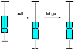
In the experiments we saw earlier, we didn't let go. We continued to stretch the material farther and farther, applying generally increasing stress until the material finally broke. Now we will look at a much more limited approach. Instead of stretching the material as far as we can, we will only stretch it a tiny bit, then release the stress so that it snaps back to its original length. We can then stress it again and release it again. We can keep repeating. Instead of a continuously increasing strain, this sample is subjected to an oscillatory strain, one that repeats in a cycle.

This approach is called dynamic mechanical analysis. We can use dynamic mechanical analysis to measure the modulus of the material. Instead of continuously moving all the way through the linear elastic region, beyond which Hooke's law breaks down, we carefully keep the sample in the Hookean region for the entire experiment. Now, one experiment should be good enough to extract the modulus, but we are letting go and doing it over again. Why?

The principle reason for running the experiment this way is to get some additional information. We can get this information because polymers don't quite follow Hooke's Law perfectly. In reality, even within the linear elastic region, the stress-strain curve is not quite linear. In the picture below, the curvature is exaggerated quite a bit, just for illustrative purposes.

Even if the relationship is not quite linear, then as we release the strain, the stress in the material should simply follow the curve back down to zero. It does not. Instead, there is a phenomenon called hysteresis at work. Hysteresis just means that a property of the material depends on how the material came to be in its current situation. In this case, Hooke's Law seems to imply that a specific sample subjected to a specific strain would experience a specific stress (or vice versa). However, it depends whether we are stretching the sample or letting it relax again. As we let the sample relax back to its initial length, the strain is different from what we saw when we were stretching it. Typically, it's lower. Again, we can see this in the curve below, where the curvature has been exaggerated.

The difference between the loading curve (when the stress was first applied) and the unloading curve (when the stress was removed) represents an energy loss. A force was applied to move a sample or a portion of a sample, some distance. When the sample snapped back the same distance, the force was unequal to the one that was initially applied. Some energy was therefore lost.

The slope of the loading curve, analogous to Young's modulus in a tensile testing experiment, is called the storage modulus, E'. The storage modulus is a measure of how much energy must be put into the sample in order to distort it. The difference between the loading and unloading curves is called the loss modulus, E". It measures energy lost during that cycling strain.

Why would energy be lost in this experiment? In a polymer, it has to do chiefly with chain flow. The resistance to deformation in a polymer comes from entanglement, including both physical crosslinks and more general occlusions as chains encounter each other while undergoing conformational changes to accommodate the new shape of the material. Once the stress is removed, the material springs back to its equilibrium shape, but there is no reason chains would have to follow the exact same conformational pathway to return to their equilibrium conformations. Because they have moved out of their original positions, they are able to follow a lower-energy pathway back to their starting point, a pathway in which there is less resistance between neighboring chains.

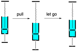
For that reason, stretching a polymer is not quite the same as stretching a mechanical spring. A "spring-and-dashpot" analogy is often invoked to describe soft materials. Whereas a spring simply bounces back to its original shape after being pulled, a dashpot does not. If you don't know what a dashpot is, picture the hydraulic arms that support the hatchback on a car when you open it upward. There is some resistance to opening the hatchback because a piston is being pulled through a hydraulic fluid as the arm stretches. When we stop lifting, the arms stay at that length, because the hydraulic fluid also resists the movement of the piston back to its original position. The dashpot has a tendency to stay put rather than spring back.

Polymers display a little of both properties. They have an elastic element, rooted in entanglement, that makes them resist deformation and return to their original shapes. They also have a viscous element, rooted in chain flow. That viscous element means that, when we distort polymeric materials, they might not return to exactly the same form as when they started out. Taken together, these behaviors are described as viscoelastic properties. Many materials have viscoelastic properties, meaning they display some aspects of elastic solids and some aspects of viscous liquids.

So far, we have concentrated on extensional deformations of materials: we have been looking at what happens when we stretch them. It's worth looking at another type of deformation because it is very commonly used in materials testing. This second approach uses shear instead of an extension to probe how the material will respond. A shear force is applied unevenly to a material so that it tilts or twists rather than stretching.

One of the reasons this approach is used so often is because it is very easy to do. A sample is sandwiched between two plates. The bottom plate is held in place while the top plate is twisted, shearing the material held in between.

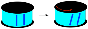
If we take a closer look at a layer of the sample, maybe at the surface, along the edge of the sandwich, we can imagine breaking it down into individual layers. Under shear strain, those layers move different amounts. The top layer, right beneath that top plate moves the most. The bottom layer, sitting on the stationary lower plate, doesn't move at all. In between, each layer moves a little further than the one beneath it. This gradation of deformation across the sample is very much like what we saw in the analysis of the viscosity of liquids. The difference is that viscosity looks at the variation of strain with time. Nevertheless, modulus in solids is roughly analogous to viscosity in liquids.

We can use this parallel plate geometry to obtain values for storage modulus and loss modulus, just like we can via an extensional geometry. The values we get are not quite the same. For this reason, modulus obtained from shear experiments is given a different symbol than modulus obtained from extensional experiments. In a shear experiment,

G = σ / ε

That means storage modulus is given the symbol G' and loss modulus is given the symbol G". Apart from providing a little more information about how the experiment was actually conducted, this distinction between shear modulus and extension modulus is important because the resulting values are quite different. In general, the value of the storage modulus obtained from an extensional experiment is about three times larger than the value of storage modulus obtained from a shear experiment.

E' = 3 G'

The reason for the difference is that extension actually involves deformation of the material in three directions. As the material is stretched in one direction (let's say it's the y-direction), in order to preserve the constant volume of the material (there is still the same amount of stuff before and after stretching), the material compresses in both the other two directions (x and z).

Problem PP8.1.

Metric prefixes are frequently encountered when reading about modulus. Rank the following units of stress from smallest to largest, and in each case provide a conversion factor to Pa.

GPa kPa MPa Pa