

3.2: Conformational analyses
- Page ID
- 527172

\( \newcommand{\vecs}[1]{\overset { \scriptstyle \rightharpoonup} {\mathbf{#1}} } \)
\( \newcommand{\vecd}[1]{\overset{-\!-\!\rightharpoonup}{\vphantom{a}\smash {#1}}} \)
\( \newcommand{\dsum}{\displaystyle\sum\limits} \)
\( \newcommand{\dint}{\displaystyle\int\limits} \)
\( \newcommand{\dlim}{\displaystyle\lim\limits} \)
\( \newcommand{\id}{\mathrm{id}}\) \( \newcommand{\Span}{\mathrm{span}}\)
( \newcommand{\kernel}{\mathrm{null}\,}\) \( \newcommand{\range}{\mathrm{range}\,}\)
\( \newcommand{\RealPart}{\mathrm{Re}}\) \( \newcommand{\ImaginaryPart}{\mathrm{Im}}\)
\( \newcommand{\Argument}{\mathrm{Arg}}\) \( \newcommand{\norm}[1]{\| #1 \|}\)
\( \newcommand{\inner}[2]{\langle #1, #2 \rangle}\)
\( \newcommand{\Span}{\mathrm{span}}\)
\( \newcommand{\id}{\mathrm{id}}\)
\( \newcommand{\Span}{\mathrm{span}}\)
\( \newcommand{\kernel}{\mathrm{null}\,}\)
\( \newcommand{\range}{\mathrm{range}\,}\)
\( \newcommand{\RealPart}{\mathrm{Re}}\)
\( \newcommand{\ImaginaryPart}{\mathrm{Im}}\)
\( \newcommand{\Argument}{\mathrm{Arg}}\)
\( \newcommand{\norm}[1]{\| #1 \|}\)
\( \newcommand{\inner}[2]{\langle #1, #2 \rangle}\)
\( \newcommand{\Span}{\mathrm{span}}\) \( \newcommand{\AA}{\unicode[.8,0]{x212B}}\)
\( \newcommand{\vectorA}[1]{\vec{#1}} % arrow\)
\( \newcommand{\vectorAt}[1]{\vec{\text{#1}}} % arrow\)
\( \newcommand{\vectorB}[1]{\overset { \scriptstyle \rightharpoonup} {\mathbf{#1}} } \)
\( \newcommand{\vectorC}[1]{\textbf{#1}} \)
\( \newcommand{\vectorD}[1]{\overrightarrow{#1}} \)
\( \newcommand{\vectorDt}[1]{\overrightarrow{\text{#1}}} \)
\( \newcommand{\vectE}[1]{\overset{-\!-\!\rightharpoonup}{\vphantom{a}\smash{\mathbf {#1}}}} \)
\( \newcommand{\vecs}[1]{\overset { \scriptstyle \rightharpoonup} {\mathbf{#1}} } \)
\(\newcommand{\longvect}{\overrightarrow}\)
\( \newcommand{\vecd}[1]{\overset{-\!-\!\rightharpoonup}{\vphantom{a}\smash {#1}}} \)
\(\newcommand{\ket}[1]{\left| #1 \right>}\)
\(\newcommand{\bra}[1]{\left< #1 \right|}\)
\(\newcommand{\braket}[2]{\left< #1 \vphantom{#2} \right| \left. #2 \vphantom{#1} \right>}\)
\(\newcommand{\braopket}[3]{\left< #1 \vphantom{#2}\vphantom{#3} \right| #2 \vphantom{#1}\vphantom{#3} \left| #3 \vphantom{#1}\vphantom{#2} \right>}\)
\(\newcommand{\qmvec}[1]{\mathbf{\vec{#1}}}\)
\(\newcommand{\op}[1]{\hat{\mathbf{#1}}}\)
\(\newcommand{\expect}[1]{\langle #1 \rangle}\)
\(\newcommand{\dfn}[1]{\emph{\textbf{#1}}}\)
\(\newcommand{\avec}{\mathbf a}\) \(\newcommand{\bvec}{\mathbf b}\) \(\newcommand{\cvec}{\mathbf c}\) \(\newcommand{\dvec}{\mathbf d}\) \(\newcommand{\dtil}{\widetilde{\mathbf d}}\) \(\newcommand{\evec}{\mathbf e}\) \(\newcommand{\fvec}{\mathbf f}\) \(\newcommand{\nvec}{\mathbf n}\) \(\newcommand{\pvec}{\mathbf p}\) \(\newcommand{\qvec}{\mathbf q}\) \(\newcommand{\svec}{\mathbf s}\) \(\newcommand{\tvec}{\mathbf t}\) \(\newcommand{\uvec}{\mathbf u}\) \(\newcommand{\vvec}{\mathbf v}\) \(\newcommand{\wvec}{\mathbf w}\) \(\newcommand{\xvec}{\mathbf x}\) \(\newcommand{\yvec}{\mathbf y}\) \(\newcommand{\zvec}{\mathbf z}\) \(\newcommand{\rvec}{\mathbf r}\) \(\newcommand{\mvec}{\mathbf m}\) \(\newcommand{\zerovec}{\mathbf 0}\) \(\newcommand{\onevec}{\mathbf 1}\) \(\newcommand{\real}{\mathbb R}\) \(\newcommand{\twovec}[2]{\left[\begin{array}{r}#1 \\ #2 \end{array}\right]}\) \(\newcommand{\ctwovec}[2]{\left[\begin{array}{c}#1 \\ #2 \end{array}\right]}\) \(\newcommand{\threevec}[3]{\left[\begin{array}{r}#1 \\ #2 \\ #3 \end{array}\right]}\) \(\newcommand{\cthreevec}[3]{\left[\begin{array}{c}#1 \\ #2 \\ #3 \end{array}\right]}\) \(\newcommand{\fourvec}[4]{\left[\begin{array}{r}#1 \\ #2 \\ #3 \\ #4 \end{array}\right]}\) \(\newcommand{\cfourvec}[4]{\left[\begin{array}{c}#1 \\ #2 \\ #3 \\ #4 \end{array}\right]}\) \(\newcommand{\fivevec}[5]{\left[\begin{array}{r}#1 \\ #2 \\ #3 \\ #4 \\ #5 \\ \end{array}\right]}\) \(\newcommand{\cfivevec}[5]{\left[\begin{array}{c}#1 \\ #2 \\ #3 \\ #4 \\ #5 \\ \end{array}\right]}\) \(\newcommand{\mattwo}[4]{\left[\begin{array}{rr}#1 \amp #2 \\ #3 \amp #4 \\ \end{array}\right]}\) \(\newcommand{\laspan}[1]{\text{Span}\{#1\}}\) \(\newcommand{\bcal}{\cal B}\) \(\newcommand{\ccal}{\cal C}\) \(\newcommand{\scal}{\cal S}\) \(\newcommand{\wcal}{\cal W}\) \(\newcommand{\ecal}{\cal E}\) \(\newcommand{\coords}[2]{\left\{#1\right\}_{#2}}\) \(\newcommand{\gray}[1]{\color{gray}{#1}}\) \(\newcommand{\lgray}[1]{\color{lightgray}{#1}}\) \(\newcommand{\rank}{\operatorname{rank}}\) \(\newcommand{\row}{\text{Row}}\) \(\newcommand{\col}{\text{Col}}\) \(\renewcommand{\row}{\text{Row}}\) \(\newcommand{\nul}{\text{Nul}}\) \(\newcommand{\var}{\text{Var}}\) \(\newcommand{\corr}{\text{corr}}\) \(\newcommand{\len}[1]{\left|#1\right|}\) \(\newcommand{\bbar}{\overline{\bvec}}\) \(\newcommand{\bhat}{\widehat{\bvec}}\) \(\newcommand{\bperp}{\bvec^\perp}\) \(\newcommand{\xhat}{\widehat{\xvec}}\) \(\newcommand{\vhat}{\widehat{\vvec}}\) \(\newcommand{\uhat}{\widehat{\uvec}}\) \(\newcommand{\what}{\widehat{\wvec}}\) \(\newcommand{\Sighat}{\widehat{\Sigma}}\) \(\newcommand{\lt}{<}\) \(\newcommand{\gt}{>}\) \(\newcommand{\amp}{&}\) \(\definecolor{fillinmathshade}{gray}{0.9}\)
Sawhorse projection and Newman projection
Multiple ways have been developed to represent organic molecules, as illustrated in Figure \(\PageIndex{1}\). Each of these helps visualize the molecule and explain certain aspects of its properties. Lewis structures, zig-zag projections or perspective drawings, and skeletal structures were described in the previous chapters. Sawhorse projection and Newman projection are described here. These, particularly the Newman projection, are helpful in the study of conformational analysis.
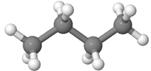 Model
 Zig-zag projection
 Skeletal structure
 Sawhorse projection
 Newman projection
Sawhorse projection is a drawing of a molecule along a \(\ce{C-C}\) bond drawn as a diagonal line, where the left-hand bottom end is the carbon near the viewer and the right-hand top end is the carbon that is further away, as illustrated in Figure \(\PageIndex{1}\).
The Newman projection is drawn as a view through a \(\ce{C-C}\) bond perpendicular to the paper, with the bonds from it to other groups as projections in the plane of the paper. The \(\ce{C}\) near the observes is shown as a dot and three groups projecting from it like in a trigonal planer geometry, while the rear \(\ce{C}\) is represented as a circle with bonds from it to other groups drawn as if projecting from behind the circle, as illustrated in Figure \(\PageIndex{1}\).
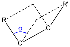
Dihedral angle or torsion angle \(\alpha\) is the clockwise angle between half-planes through two sets of three atoms, e.g., the half-planes defined by \(\ce{R-C-C}\) and \(\ce{R'-C-C}\) in Figure \(\PageIndex{2}\), having two atoms (\(\ce{C-C}\) in this case) in common.
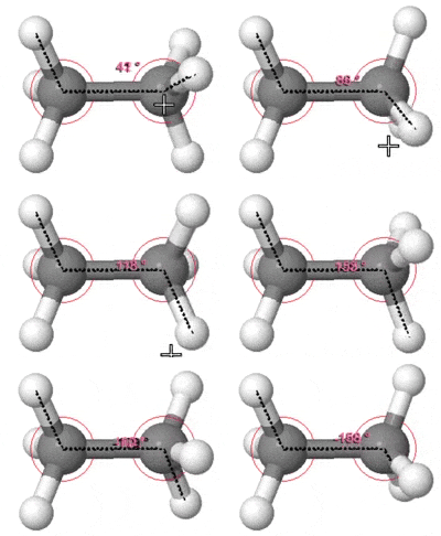 For example, the dihedral angle between \(\ce{-CH3}\) on the front \(\ce{C}\) and \(\ce{-CH3}\) on the front \(\ce{C}\) is 180\(^\circ\); and \(\ce{-CH3}\) on the front \(\ce{C}\) and any of the \(\ce{-H}\) on the front \(\ce{C}\) 60\(^\circ\). Rotation around a single bond results in different conformations, as illustrated for ethane \(\ce{CH3-CH3}\) on the right margin. These conformations are easier to view using Newman projections. Particularly, converting one conformation to another is easier to draw by keeping the form \(\ce{C}\) fixed and rotating the rear \(\ce{C}\) in a Newman projection, i.e., by rotating the wheel.
Conformational analysis of ethane
 Rotation occurs around \(\ce{C-C}\) bond in ethane, resulting in various conformations, as shown by simulation in the right margin above. However, the rotation is not entirely free; three energy barriers limit its movement. Therefore, as the dihedral angle gradually changes from 0\(^\circ\) to 360\(^\circ\), the relative potential energy of the molecule goes through local minima to local maxima, often at intervals of 60\(^\circ\).
The conformation of ethane in which a \(\ce{H}\) on the front \(\ce{C}\) in a Newman projection is at a dihedral angle of 0\(^\circ\) from the nearest \(\ce{H}\) on the rear \(\ce{C}\) is called eclipsed. The one in which they are at 60\(^\circ\) is called a staggard, as illustrated in the figure on the right margin.
The eclipsed conformation of ethane corresponds to the energy maximum. As the dihedral angle gradually increases from 0\(^\circ\), the energy gradually decreases, reaching a minimum at 60\(^\circ\), followed by a gradual increase reaching a maximum again at 120\(^\circ\). This cycle repeats, resulting in a sinusoidal curve of potential energy versus dihedral angle, as shown in Figure \(\PageIndex{3}\).
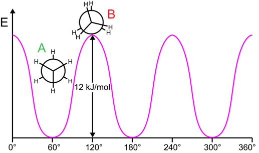
The energy difference between the staggered conformation of ethane at the energy minima and the eclipsed conformation at the energy maxima is 12 kJ/mol. Since there are three \(\ce{H}\) to \(\ce{H}\) eclipsing interactions, each \(\ce{H}\) to \(\ce{H}\) eclipsing costs 4 kJ/mol.
The following factors contribute to the stabilization or destabilization of the conformation.
- Destabilization due to electrostatic repulsion between the identical charge dipoles nearby in eclipsed conformation,
- destabilization due to steric repulsion, i.e., physical repulsion due to electron cloud on one group penetrating the electron cloud space of the other when they are nearby in eclipsed conformation, and
- stabilization due to hyperconjugation, i.e., an overlap of a \(\sigma\)-bond on one atom with an antibonding orbital on the neighboring atom in staggered conformation.
These factors are illustrated in Figure \(\PageIndex{4}\) for the case of ethane.

Note that the hyperconjugation is a resonance involving \(\sigma\)-bond. In the case of eclipsed ethane, the staggered conformation is stabilized by hyperconjugation, i.e., an overlap between a \(\sigma\)-bond and an antibonding orbital. The hyperconjugation is lost as the orbitals move out of alignment in the eclipsed conformation. Hyperconjugation and static repulsion could be the reason for destabilising the eclipsed conformation, also referred to as an eclipsing strain. Steric repulsion is not responsible for it because the size of \(\ce{-H}\) substituent is small.
 The potential energy versus dihedral angle curve of propane is similar to that of ethane, except that the difference between the staggered and eclipsed conformation is 14 kJ/mol in propane. There are two \(\ce{H}\) to \(\ce{H}\) eclipsing interactions and one \(\ce{CH3}\) to \(\ce{H}\) eclipsing in the staggered conformation of propane, as shown in the figure on the right margin. Two \(\ce{H}\) to \(\ce{H}\) eclipsing interactions are 4 kJ/mol each, the same in ethane and propane, which means \(\ce{CH3}\) to \(\ce{H}\) eclipsing in propane is 6 kJ/mole resulting in a total of 14 kJ/mole in propane. Since \(\ce{-CH3}\) is bulkier than \(\ce{-H}\), steric repulsion, also called steric strain, contributes to the eclipsing strain of propane.
Conformational analysis of butane

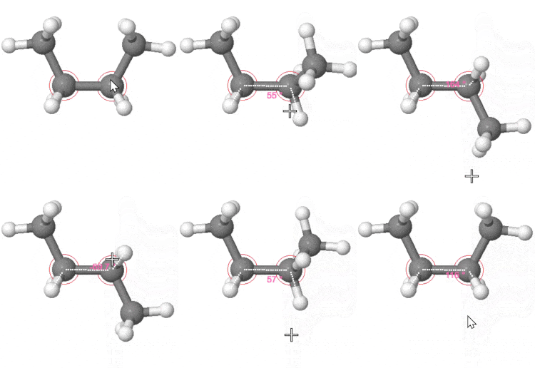 The conformational analysis of butane \(\ce{CH3CH2CH2CH3}\) is discussed concerning rotation around \(\ce{C\text{2}-C\text{3}}\) bond, as shown in the simulation on the left margin. The most stable conformation is illustrated on the right margin. This is a staggered conformation of lowest energy with the bulky \(\ce{-CH3}\) groups farthest apart at 180\(^\circ\), which is labeled A in the relative energy vs. torsion angle curve shown in Figure \(\PageIndex{5}\). It is referred to as anti-conformation. A 60\(^\circ\) rotation converts it to an eclipsed conformation labeled C in the figure. It has one \(\ce{H}\) to \(\ce{H}\) eclipsing interaction of 4 kJ/mole and two \(\ce{H}\) to \(\ce{CH3}\) eclipsing interactions of 6 kJ/mol each, which totals to 16 kJ/mol higher energy relative to the anti-confirmation. A further 60\(^\circ\) rotation converts the eclipsed conformation to another staggered conformation called gauche-conformation, labeled B. It is at a local energy minimum but 3.8 kJ/mol higher than the anti-conformation. The gauche conformation has the bulky \(\ce{-CH3}\) groups at a 60\(^\circ\) torsion angle where they are close enough to cause some steric repulsion between each other. Another 60\(^\circ\) rotation converts the gauche-conformation to an eclipsed conformation called cis, labeled D, in which the bulky \(\ce{-CH3}\) groups are eclipsing each other. The cis-conformation is 19 kJ/mole higher than the anti-conformation. There are two \(\ce{H}\) to \(\ce{H}\) eclipsing interactions of 4 kJ/mol each, and the remaining 11 kJ/mol is due to \(\ce{CH3}\) to \(\ce{CH3}\) eclipsing interaction. This cis-conformation, labeled C, is 3 kJ/mol higher in energy than the other eclipsed conformation, labeled B, and it is the highest energy conformation of butane. These conformations repeat at an interval of 60\(^\circ\) torsion angles, as illustrated in Figure \(\PageIndex{5}\).

Figure \(\PageIndex{6}\) shows the models of the conformations, labeled A, B, C, and D in Figure \(\PageIndex{5}\), with the van der Wall electron cloud spaces shown. It also provides a summary of the nomenclature associated with the conformations.
 A: antiperiplanar, anti or trans
 B: gauche synclinal, or skew
 C: eclipsed
 D: synperiplanar or cis.
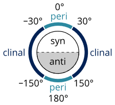 E: nomenclature of conformations
- Conformations corresponding to local minima on the potential energy curve, e.g., anti- and gauche-conformations in the case of butane, are called conformational isomers or conformers.
- The conformations corresponding to the local maxima on the energy curve, such as the eclipsed conformations in the case of butane, are transition states between conformational isomers that have a fleeting existence.
It can be calculated form Figure \(\PageIndex{4}\) and Figure \(\PageIndex{6}\) that each
Conformations of cycloalkanes
If a cycloalkane is a planar ring, there will be two kinds of strain:
- angle strain, i.e., the strain caused by bending the bond angles from the ideal tetrahedral bond angles of 109.5\(\circ\), and
- eclipsing strains between a pair of \(\ce{H}\) on each \(\ce{C}\) with pairs of \(\ce{H's}\) on the two neighboring carbons.
 Cyclopropane is a planar ring with bond angles reduced to 60\(^\circ\) and three \(\ce{H}\) to \(\ce{H}\) eclipsing interaction on the top face and three on the bottom face, as shown by red dotted lines in the figure on the right margin. The planar conformation of cyclopropane with the eclipsing interactions between \(\ce{H's}\) can be seen in the interactive model in Figure \(\PageIndex{7}\). The overall strain on a cyclopropane is ~120 kJ/mol, of which 24 kJ/mol (6 x 4 = 24 kJ/mol) is accounted for by the \(\ce{H}\) eclipsing strain and the remaining 96 kJ/mol is due to angle strain. Cyclopropane is the most strained cycloalkane.
Figure \(\PageIndex{7}\): Interactive models of cyclopropane (left), cyclobutane (middle), and cyclopentane (right) The model can be enlarged by two fingers gesturing the touchpad or right-clicking and moving, and rotated by swiping one finger in the image area or left-clicking the mouse and moving (Copyright: public domain).
A planar cyclobutane would would be square with 90\(^\circ\) bond angles and 8 \(\ce{H}\) to \(\ce{H}\) eclipsing. The actual conformation of cyclobutane is puckered confirmation as shown in the interactive model in Figure \(\PageIndex{7}\). The puckered conformation increases angle strain by reducing angles to 88\(^\circ\) but significantly reduces the \(\ce{H}\) to \(\ce{H}\) eclipsing strain, resulting in an overall ring strain of ~110 kJ/mol.
A planar cyclopentane would be a pentagon with bond angles of 108\(\circ\), i.e., close to the regular value of 109.5o, but ten \(\ce{H}\) to \(\ce{H}\) eclipsing interaction that would be 40 kJ/mole (10 x 4 = 40 kJ/mol) overall strain. The actual conformation of cyclopentane is puckered, shown in the interactive model in Figure \(\PageIndex{7}\). The puckered conformation slightly increases angle strain but significantly reduces eclipsing strain, resulting in an overall strain of ~25 kJ/mol. Four of the \(\ce{C}\) 's of cyclopentane are almost in one plane, and the fifth is raised, giving it an envelope shape, also known as an envelope conformation. The raised \(\ce{C}\) position keeps shifting between the five ring \(\ce{C's}\), and the resulting five envelop shape isomers exist in an equilibrium mixture. Cyclopentane is one of the most common ring structures found in nature due to its low angle strain. For example, ribose, a sugar that is a component of DNA monomers, and fructose, or fruit sugar, are five-membered rings.
Figure \(\PageIndex{8}\): Interactive models of cyclohexane (left), cyclooctane (middle), and cyclopentahexane (right) The model can be enlarged by two fingers gesturing the touchpad or right-clicking and moving, and rotated by swiping one finger in the image area or left-clicking the mouse and moving (Copyright: public domain).
 A planar cyclohexane would be a hexagon with all \(\ce{C-C-C}\) bond angles expanded to 120\(^\circ\) and 12 \(\ce{H}\) to \(\ce{H}\) eclipsing interactions. The actual conformations of cyclohexane are bent, with the most stable conformation resembling a chair, known as the chair conformation, as shown in the figure on the right margin and the interactive model in Figure \(\PageIndex{8}\). In the chair conformation of cyclohexane, all bond angles are close to the tetrahedral value of 109.5\(^\circ\) and all \(\ce{H's}\) are staggered with no ring strain. Cyclohexane is the most common ring structure found in nature due to its zero ring strain. For example, glucose -the most common monosaccharide (sugar) is six-membered rings. Starch, a carbohydrate component of food, and cellulose, a major component of wood, are made of glucose units.
 Medium-size rings (7-13 \(\ce{C's}\)) can pucker or bend to minimize angle strain, as shown in Figure \(\PageIndex{8}\) Still, some transannular strain, i.e., steric repulsion between groups attached to non-adjacent ring atoms, appears between groups on some \(\ce{C's}\) with other groups at a distance across the ring.
 For example, the figure on the right margin highlights the transannular strain between two \(\ce{H's}\) with a red oval shape in the lowest energy conformation of cyclooctane (Copyright; public domain). In larger rings (14 or more \(\ce{C's}\)), there is little or no ring strain because they are more flexible and can acquire conformations with minimal angle strain, eclipsing strain, and transannular strain. The figure on the left margin summarizes the strain energy concerning the ring size trend (Copyright; Public domain).