5.5: Asymmetric Centers and Stereocenters
- Page ID
- 13849
\( \newcommand{\vecs}[1]{\overset { \scriptstyle \rightharpoonup} {\mathbf{#1}} } \)
\( \newcommand{\vecd}[1]{\overset{-\!-\!\rightharpoonup}{\vphantom{a}\smash {#1}}} \)
\( \newcommand{\id}{\mathrm{id}}\) \( \newcommand{\Span}{\mathrm{span}}\)
( \newcommand{\kernel}{\mathrm{null}\,}\) \( \newcommand{\range}{\mathrm{range}\,}\)
\( \newcommand{\RealPart}{\mathrm{Re}}\) \( \newcommand{\ImaginaryPart}{\mathrm{Im}}\)
\( \newcommand{\Argument}{\mathrm{Arg}}\) \( \newcommand{\norm}[1]{\| #1 \|}\)
\( \newcommand{\inner}[2]{\langle #1, #2 \rangle}\)
\( \newcommand{\Span}{\mathrm{span}}\)
\( \newcommand{\id}{\mathrm{id}}\)
\( \newcommand{\Span}{\mathrm{span}}\)
\( \newcommand{\kernel}{\mathrm{null}\,}\)
\( \newcommand{\range}{\mathrm{range}\,}\)
\( \newcommand{\RealPart}{\mathrm{Re}}\)
\( \newcommand{\ImaginaryPart}{\mathrm{Im}}\)
\( \newcommand{\Argument}{\mathrm{Arg}}\)
\( \newcommand{\norm}[1]{\| #1 \|}\)
\( \newcommand{\inner}[2]{\langle #1, #2 \rangle}\)
\( \newcommand{\Span}{\mathrm{span}}\) \( \newcommand{\AA}{\unicode[.8,0]{x212B}}\)
\( \newcommand{\vectorA}[1]{\vec{#1}} % arrow\)
\( \newcommand{\vectorAt}[1]{\vec{\text{#1}}} % arrow\)
\( \newcommand{\vectorB}[1]{\overset { \scriptstyle \rightharpoonup} {\mathbf{#1}} } \)
\( \newcommand{\vectorC}[1]{\textbf{#1}} \)
\( \newcommand{\vectorD}[1]{\overrightarrow{#1}} \)
\( \newcommand{\vectorDt}[1]{\overrightarrow{\text{#1}}} \)
\( \newcommand{\vectE}[1]{\overset{-\!-\!\rightharpoonup}{\vphantom{a}\smash{\mathbf {#1}}}} \)
\( \newcommand{\vecs}[1]{\overset { \scriptstyle \rightharpoonup} {\mathbf{#1}} } \)
\( \newcommand{\vecd}[1]{\overset{-\!-\!\rightharpoonup}{\vphantom{a}\smash {#1}}} \)
\(\newcommand{\avec}{\mathbf a}\) \(\newcommand{\bvec}{\mathbf b}\) \(\newcommand{\cvec}{\mathbf c}\) \(\newcommand{\dvec}{\mathbf d}\) \(\newcommand{\dtil}{\widetilde{\mathbf d}}\) \(\newcommand{\evec}{\mathbf e}\) \(\newcommand{\fvec}{\mathbf f}\) \(\newcommand{\nvec}{\mathbf n}\) \(\newcommand{\pvec}{\mathbf p}\) \(\newcommand{\qvec}{\mathbf q}\) \(\newcommand{\svec}{\mathbf s}\) \(\newcommand{\tvec}{\mathbf t}\) \(\newcommand{\uvec}{\mathbf u}\) \(\newcommand{\vvec}{\mathbf v}\) \(\newcommand{\wvec}{\mathbf w}\) \(\newcommand{\xvec}{\mathbf x}\) \(\newcommand{\yvec}{\mathbf y}\) \(\newcommand{\zvec}{\mathbf z}\) \(\newcommand{\rvec}{\mathbf r}\) \(\newcommand{\mvec}{\mathbf m}\) \(\newcommand{\zerovec}{\mathbf 0}\) \(\newcommand{\onevec}{\mathbf 1}\) \(\newcommand{\real}{\mathbb R}\) \(\newcommand{\twovec}[2]{\left[\begin{array}{r}#1 \\ #2 \end{array}\right]}\) \(\newcommand{\ctwovec}[2]{\left[\begin{array}{c}#1 \\ #2 \end{array}\right]}\) \(\newcommand{\threevec}[3]{\left[\begin{array}{r}#1 \\ #2 \\ #3 \end{array}\right]}\) \(\newcommand{\cthreevec}[3]{\left[\begin{array}{c}#1 \\ #2 \\ #3 \end{array}\right]}\) \(\newcommand{\fourvec}[4]{\left[\begin{array}{r}#1 \\ #2 \\ #3 \\ #4 \end{array}\right]}\) \(\newcommand{\cfourvec}[4]{\left[\begin{array}{c}#1 \\ #2 \\ #3 \\ #4 \end{array}\right]}\) \(\newcommand{\fivevec}[5]{\left[\begin{array}{r}#1 \\ #2 \\ #3 \\ #4 \\ #5 \\ \end{array}\right]}\) \(\newcommand{\cfivevec}[5]{\left[\begin{array}{c}#1 \\ #2 \\ #3 \\ #4 \\ #5 \\ \end{array}\right]}\) \(\newcommand{\mattwo}[4]{\left[\begin{array}{rr}#1 \amp #2 \\ #3 \amp #4 \\ \end{array}\right]}\) \(\newcommand{\laspan}[1]{\text{Span}\{#1\}}\) \(\newcommand{\bcal}{\cal B}\) \(\newcommand{\ccal}{\cal C}\) \(\newcommand{\scal}{\cal S}\) \(\newcommand{\wcal}{\cal W}\) \(\newcommand{\ecal}{\cal E}\) \(\newcommand{\coords}[2]{\left\{#1\right\}_{#2}}\) \(\newcommand{\gray}[1]{\color{gray}{#1}}\) \(\newcommand{\lgray}[1]{\color{lightgray}{#1}}\) \(\newcommand{\rank}{\operatorname{rank}}\) \(\newcommand{\row}{\text{Row}}\) \(\newcommand{\col}{\text{Col}}\) \(\renewcommand{\row}{\text{Row}}\) \(\newcommand{\nul}{\text{Nul}}\) \(\newcommand{\var}{\text{Var}}\) \(\newcommand{\corr}{\text{corr}}\) \(\newcommand{\len}[1]{\left|#1\right|}\) \(\newcommand{\bbar}{\overline{\bvec}}\) \(\newcommand{\bhat}{\widehat{\bvec}}\) \(\newcommand{\bperp}{\bvec^\perp}\) \(\newcommand{\xhat}{\widehat{\xvec}}\) \(\newcommand{\vhat}{\widehat{\vvec}}\) \(\newcommand{\uhat}{\widehat{\uvec}}\) \(\newcommand{\what}{\widehat{\wvec}}\) \(\newcommand{\Sighat}{\widehat{\Sigma}}\) \(\newcommand{\lt}{<}\) \(\newcommand{\gt}{>}\) \(\newcommand{\amp}{&}\) \(\definecolor{fillinmathshade}{gray}{0.9}\)To better understand the molecular origins of the ideal gas law,
\[PV=nRT\]
the basics of the Kinetic Molecular Theory of Gases (KMT) should be understood. This model is used to describe the behavior of gases. More specifically, it is used to explain macroscopic properties of a gas, such as pressure and temperature, in terms of its microscopic components, such as atoms. Like the ideal gas law, this theory was developed in reference to ideal gases, although it can be applied reasonably well to real gases.
In order to apply the kinetic model of gases, five assumptions are made:
- Gases are made up of particles with no defined volume but with a defined mass. In other words their volume is miniscule compared to the distance between themselves and other molecules.
- Gas particles undergo no intermolecular attractions or repulsions. This assumption implies that the particles possess no potential energy and thus their total energy is simply equal to their kinetic energies.
- Gas particles are in continuous, random motion.
- Collisions between gas particles are completely elastic. In other words, there is no net loss or gain of kinetic energy when particles collide.
- The average kinetic energy is the same for all gases at a given temperature, regardless of the identity of the gas. Furthermore, this kinetic energy is proportional to the absolute temperature of the gas.
Temperature and KMT
The last assumption can be written in equation form as:
\[KE = \dfrac{1}{2}mv^2 = \dfrac{3}{2}k_BT\]
where
- \(k_B\) is Boltzmann's constant (kB = 1.381×10⁻²³ m2 kg s-2 K-1) and
- \(T\) is the absolution temperature (in Kelvin)
This equation says that the speed of gas particles is related to their absolute temperature. In other words, as their temperature increases, their speed increases, and finally their total energy increases as well. However, it is impossible to define the speed of any one gas particle. As such, the speeds of gases are defined in terms of their root-mean-square speed.
Pressure and KMT
The macroscopic phenomena of pressure can be explained in terms of the kinetic molecular theory of gases. Assume the case in which a gas molecule (represented by a sphere) is in a box, length L (Figure 1). Through using the assumptions laid out above, and considering the sphere is only moving in the x-direction, we can examine the instance of the sphere colliding elastically with one of the walls of the box.
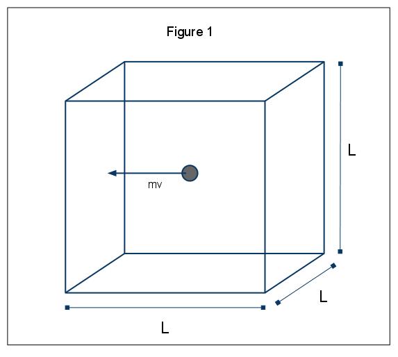
The momentum of this collision is given by p=mv, in this case p=mvx, since we are only considering the x dimension. The total momentum change for this collision is then given by
\[mv_x - m(-v_x) = 2mv_x\]
Given that the amount of time it takes between collisions of the molecule with the wall is L/vx we can give the frequency of collisions of the molecule against a given wall of the box per unit time as vx/2L. One can now solve for the change in momentum per unit of time:
\[(2mv_x)(v_x/2L) = mv_x^2/L\]
Solving for momentum per unit of time gives the force exerted by an object (F=ma=p/time). With the expression that F=mvx2/L one can now solve for the pressure exerted by the molecular collision, where area is given as the area of one wall of the box, A=L2:
\[P=\dfrac{F}{A}\]
\[P=\dfrac{mv_x^2}{[L(L^2)}\]
The expression can now be written in terms of the pressure associated with collisions from N number of molecules:
\[P=\dfrac{Nmv_x^2}{V}\]
This expression can now be adjusted to account for movement in the x, y and z directions by using mean-square velocity for three dimensions and a large value of N. The expression now is written as:
\[P={\dfrac{Nm\overline{v}^2}{3V}}\]
This expression now gives pressure, a macroscopic quality, in terms of atomic motion. The significance of the above relationship is that pressure is proportional to the mean-square velocity of molecules in a given container. Therefore, as molecular velocity increases so does the pressure exerted on the container.
References
- Oxtoby, Gillis and Campion. Principles of Modern Chemistry. 6th Edition. California: Thomson Brooks/Cole. 2008.
- Chang, Raymond. Physical Chemistry for the Biosciences. California: University Science Books. 2005.
Contributors and Attributions
- Sevini Shahbaz, Andrew Cooley