
27.4: Why Spin-Spin Splitting?
- Page ID
- 22379

In Section 9-10G, we outlined the structural features that lead to observation of spin-spin splitting in the NMR spectra of organic compounds. Rules for predicting the multiplicities and intensities of spin-spin splitting patterns also were discussed. However, we did not discuss the underlying basis for spin-spin splitting, which involves perturbation of the nuclear magnetic energy levels shown in Figure 9-21 by magnetic interaction between the nuclei. You may wish to understand more about the origin of spin-spin splitting than is provided by the rules for correlating and predicting spin-spin splitting given previously, but having a command of what follows is not necessary to the qualitative use of spin-spin splitting in structural analysis. However, it will provide you with an understanding of the origins of the line spacings and line multiplicities. We will confine our attention to protons, but the same considerations apply to other nuclei (\(\ce{^{13}C}\), \(\ce{^{15}N}\), \(\ce{^{19}F}\), and \(\ce{^{31}P}\)) that have the spin \(I = \frac{1}{2}\). The main differences between proton-proton splittings and those of other nuclei are in the magnitudes of the splitting constants (\(J\) values) and their variation with structure.
Why does splitting occur? Let us start by comparing the two-proton systems of \(7\) and \(8\):
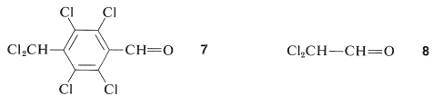
The protons in each compound will have the shift differences typical of \(\ce{Cl_2CH}-\) and \(\ce{-CHO}\) and, at \(60 \: \text{MHz}\), can be expected from the data in Table 9-4 and Equation 9-4 to be observed at about \(350 \: \text{Hz}\) and \(580 \: \text{Hz}\), respectively, from TMS. Now consider a frequency-sweep experiment\(^4\) arranged so that the \(\ce{-CH=O}\) proton will come into resonance first.
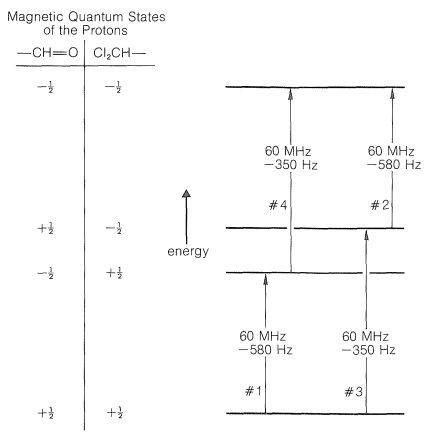
For \(7\) the two protons are separated by seven bonds in all (five carbon-carbon and two carbon-hydrogen bonds), thus we expect spin-spin splitting to be negligible. We can construct an energy diagram (Figure 27-5) for the magnetic energies of the possible states of two protons at \(60 \: \text{MHz}\) with the aid of Figure 9-24. (If this diagram is not clear to you, we suggest you review Section 9-10A before proceeding.)
Now consider \(\ce{Cl_2CH-CH=O}\), in which the protons are in close proximity to one another, three bonds apart. Each of these protons has a magnetic field and two possible magnetic states that correspond to a compass needle pointing either north or south (see Figure 9-21). The interactions between a north-north set of orientations (\(+\frac{1}{2}\), \(+\frac{1}{2}\) or \(\rightrightarrows\)) of the two protons or a south-south set (\(-\frac{1}{2}\), \(-\frac{1}{2}\) or \(\leftleftarrows\)) will make these states less stable, whereas the interactions between either a north-south (\(+\frac{1}{2}\), \(-\frac{1}{2}\) or \(\rightleftarrows\)) or a south-north (\(-\frac{1}{2}\), \(+\frac{1}{2}\) or \(\leftrightarrows\)) orientation will make these states more stable. Why? Because north-south or south-north orientations of magnets attract each other, whereas north-north or south-south repel each other.\(^5\) Let us suppose the \(+\frac{1}{2}\), \(+\frac{1}{2}\) or \(-\frac{1}{2}\), \(-\frac{1}{2}\) orientations are destabilized by \(1.25 \: \text{Hz}\). The \(+\frac{1}{2}\), \(-\frac{1}{2}\) or \(-\frac{1}{2}\), \(+\frac{1}{2}\) states must then be stabilized \(1.25 \: \text{Hz}\). Correction of the energy levels and the transition energies for these spin-spin magnetic interactions is shown in Figure 27-6.
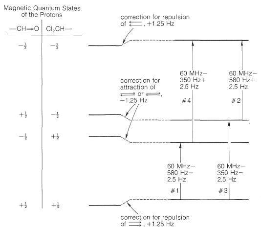
There are four possible combinations of the magnetic quantum numbers of the two protons of \(\ce{CHCl_2CHO}\), as shown in Figure 27-6. Because the differences in energy between the magnetic states corresponding to these four combinations is very small (see Section 9-10A), there will be almost equal numbers of \(\ce{CHCl_2CHO}\) molecules with the \(\left( +\frac{1}{2}, \: +\frac{1}{2} \right)\), \(\left( -\frac{1}{2}, \: +\frac{1}{2} \right)\), \(\left( +\frac{1}{2}, \: -\frac{1}{2} \right)\), and \(\left( -\frac{1}{2}, \: -\frac{1}{2} \right)\) spin combinations. The transitions shown in Figure 27-6 will be observed for those molecules with the two protons in the \(\left( +\frac{1}{2}, \: +\frac{1}{2} \right)\) state going to the \(\left( -\frac{1}{2}, \: +\frac{1}{2} \right)\) state or for the molecules with \(\left( +\frac{1}{2}, \: +\frac{1}{2} \right)\) to \(\left( +\frac{1}{2}, \: -\frac{1}{2} \right)\) as well as from \(\left( -\frac{1}{2}, \: +\frac{1}{2} \right) \rightarrow \left( -\frac{1}{2}, \: -\frac{1}{2} \right)\) and \(\left( +\frac{1}{2}, \: -\frac{1}{2} \right) \rightarrow \left( -\frac{1}{2}, \: -\frac{1}{2} \right)\).\(^6\) It is very important to remember that the transitions shown in Figure 27-6 involve molecules that have protons in different spin states, and by the uncertainty principle (Section 27-1) the lifetimes of these spin states must be long if sharp resonance lines are to be observed.
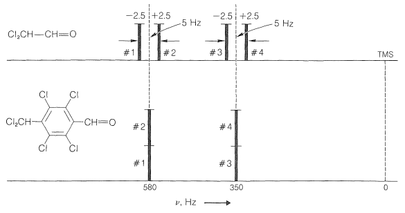
Now if we plot the energies of the transitions shown in Figures 27-5 and 27-6, we get the predicted line positions and intensities of Figure 27-7. Four lines in two equally spaced pairs appear for \(\ce{Cl_CH-CH=O}\), as expected from the naive rules for spin-spin splitting.
A harder matter to explain, and what indeed is beyond the scope of this book to explain, is why, as the chemical shift is decreased at constant spin-spin interactions, the outside lines arising from a system of two nuclei of the type shown in Figure 27-7 become progressively weaker in intensity, as shown in Figure 9-44. Furthermore, the inside lines move closer together, become more intense, and finally coalesce into a single line as the chemical-shift difference, \(\delta\), approaches zero. All we can give you here is the proposition that the outside lines become "forbidden" by spectroscopic selection rules as the chemical shift approaches zero. At the same time, the transitions leading to the inside lines become more favorable so that the integrated peak intensity of the overall system remains constant.\(^7\)
In a similar category of difficult explanations is the problem of why second-order splittings are observed, as in Figure 9-32. The roots of the explanation again lie in quantum mechanics which we cannot cover here, but which do permit very precise quantitative prediction and also qualitative understanding.\(^7\) The important point to remember is that whenever the chemical shifts and couplings begin to be of similar magnitude, you can expect to encounter NMR spectra that will have more lines and lines in different positions than you would expect from the simple treatment we developed in this chapter and in Chapter 9.
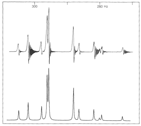
In extreme cases, such as with the protons of 4-deuterio-1-buten-3-yne, shown in Figure 27-8, none of the line positions or spacings correspond directly to any one chemical shift or spin-spin coupling. However, it is important to recognize that such spectra by no means defy analysis and, as also is seen in Figure 27-8, excellent correspondence can be obtained between calculated and observed line positions and intensities by using appropriate chemical shift and coupling parameters. However, such calculations are numerically laborious and are best made with the aid of a high-speed digital computer.
\(^4\)We will use frequency sweep simply because it is easier to talk about energy changes in frequency units. However, the same arguments will hold for a field-sweep experiment.
\(^5\)Such interactions with simple magnets will average to zero if the magnets are free to move around each other at a fixed distance. However, when electrons are between the magnets, as they are for magnetic nuclei in molecules, a small residual stabilization (or destabilization) is possible. Because these magnetic interactions are "transmitted" through the bonding electrons, we can understand in principle why it is that the number of bonds between the nuclei, the bond angles, conjugation, and so on, is more important than just the average distance between the nuclei in determining the size of the splittings.
\(^6\)The transitions \(\left( +\frac{1}{2}, \: +\frac{1}{2} \right) \rightarrow \left( -\frac{1}{2}, \: -\frac{1}{2} \right)\) and \(\left( -\frac{1}{2}, \: +\frac{1}{2} \right) \rightarrow \left( +\frac{1}{2}, \: -\frac{1}{2} \right)\) are in quantum-mechanical terms known as "forbidden" transitions and are not normally observed. Notice that the net spin changes by \(\pm\)1 for "allowed" transitions.
\(^7\)A relatively elementary exposition of these matters is available in J. D. Roberts, An Introduction to Spin-Spin Splitting in High-Resolution Nuclear Magnetic Resonance Spectra, W. A. Benjamin, Inc., Menlo Park, Calif., 1961.
Contributors and Attributions
John D. Robert and Marjorie C. Caserio (1977) Basic Principles of Organic Chemistry, second edition. W. A. Benjamin, Inc. , Menlo Park, CA. ISBN 0-8053-8329-8. This content is copyrighted under the following conditions, "You are granted permission for individual, educational, research and non-commercial reproduction, distribution, display and performance of this work in any format."