6.2: Hydrogenlike Atomic Orbitals

Last updated
Save as PDF

Page ID: 22182

\( \newcommand{\vecs}[1]{\overset { \scriptstyle \rightharpoonup} {\mathbf{#1}} } \) \( \newcommand{\vecd}[1]{\overset{-\!-\!\rightharpoonup}{\vphantom{a}\smash {#1}}} \)\(\newcommand{\id}{\mathrm{id}}\) \( \newcommand{\Span}{\mathrm{span}}\) \( \newcommand{\kernel}{\mathrm{null}\,}\) \( \newcommand{\range}{\mathrm{range}\,}\) \( \newcommand{\RealPart}{\mathrm{Re}}\) \( \newcommand{\ImaginaryPart}{\mathrm{Im}}\) \( \newcommand{\Argument}{\mathrm{Arg}}\) \( \newcommand{\norm}[1]{\| #1 \|}\) \( \newcommand{\inner}[2]{\langle #1, #2 \rangle}\) \( \newcommand{\Span}{\mathrm{span}}\) \(\newcommand{\id}{\mathrm{id}}\) \( \newcommand{\Span}{\mathrm{span}}\) \( \newcommand{\kernel}{\mathrm{null}\,}\) \( \newcommand{\range}{\mathrm{range}\,}\) \( \newcommand{\RealPart}{\mathrm{Re}}\) \( \newcommand{\ImaginaryPart}{\mathrm{Im}}\) \( \newcommand{\Argument}{\mathrm{Arg}}\) \( \newcommand{\norm}[1]{\| #1 \|}\) \( \newcommand{\inner}[2]{\langle #1, #2 \rangle}\) \( \newcommand{\Span}{\mathrm{span}}\)\(\newcommand{\AA}{\unicode[.8,0]{x212B}}\)

With the modern concept of a hydrogen atom we do not visualize the orbital electron traversing a simple planetary orbit. Rather, we speak of an atomic orbital, in which there is only a probability of finding the electron in a particular volume a given distance and direction from the nucleus. The boundaries of such an orbital are not distinct because there always remains a finite, even if small, probability of finding the electron relatively far from the nucleus.

There are several discrete atomic orbitals available to the electron of a hydrogen atom. These orbitals differ in energy, size, and shape, and exact mathematical descriptions for each are possible. Following is a qualitative description of the nature of some of the hydrogen atomic orbitals.

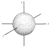
The most stable or ground state of a hydrogen atom is designated \(1s\).\(^1\) In the \(1s\) state the electron is, on the average, closest to the nucleus (i.e., it is the state with the smallest atomic orbital). The \(1s\) orbital is spherically symmetrical. This means that the probability of finding the electron at a given distance \(r\) from the nucleus is independent of the direction from the nucleus. We shall represent the \(1s\) orbital as a sphere centered on the nucleus with a radius such that the probability of finding the electron within the boundary surface is high (0.80 to 0.95); see Figure 6-1. This may seem arbitrary, but an orbital representation that would have a probability of 1 for finding the electron within the boundary surface would have an infinite radius. The reason is that there is a finite, even if small, probability of finding the electron at any given distance from the nucleus. The boundary surfaces we choose turn out to have sizes consistent with the distances between the nuclei of bonded atoms.

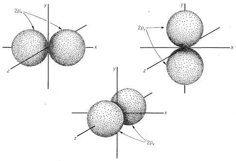
The \(2s\) orbital is very much like the \(1s\) orbital except that it is larger and therefore more diffuse, and it has a higher energy. For principal quantum number 2, there are also three orbitals of equal energies called \(2p\) orbitals, which have different geometry than the \(s\) orbitals. These are shown in Figure

Atom represented by a sphere that is white with small black dots. Vertical line going through sphere represents y axis. Horizontal line going through sphere represents x axis. Line going diagonally up through the sphere represents z axis. — Figure 6-1: Representation of the hydrogen \(1s\) orbital

6-2, in which we see that the respective axes passing through the tangent spheres of the three \(p\) orbitals lie at right angles to one another. The \(p\) orbitals are not spherically symmetrical.

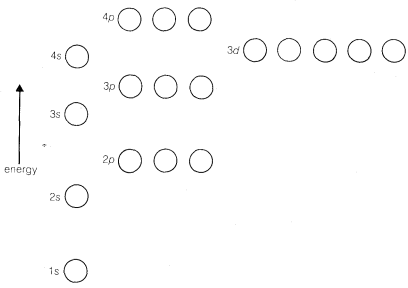
The \(3s\) and \(3p\) states are similar to the \(2s\) and \(2p\) states but are of higher energy. The \(3d\), \(4d\), \(4f\), \(\cdots\), orbitals have still higher energies and quite different geometries; they are not important for bonding in most organic substances, at least for carbon compounds with hydrogen and elements in the first main row (\(Li\)-\(Ne\)) of the periodic table. The sequence of orbital energies is shown in Figure 6-3.

Left: Two atoms next to each other and slightly touching lined up on the x axis. Labeled 2 p x. Middle: Two atoms lined up on the z axis. Labeled 2 p z. Right: Two atoms lined up on the y axis. Labeled 2 p y. — Figure 6-2: The shapes and orientations of the three \(2p\) orbitals of a hydrogen atom. Notice that \(p\) orbitals have two lobes, one on each side of the nucleus.

Energy diagram with various orbitals. Vertical arrow labeled energy shows that the higher the atom, the higher the energy. Four circles (conveying an atom) in the s orbitals which are the farthest to the left. One atom in each of the four s orbitals labeled one (lowest) through four (highest). Three atoms in each of the three p orbitals which are in the middle. Orbitals labeled 2 (lowest) through 4 (highest). The rightmost orbital is the d orbital. One level (3 D) with five atoms. — Figure 6-3: Schematic diagram of the relative energies of the hydrogen-like atomic orbitals

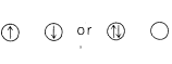
The famous Pauli exclusion principle states that no more than two elections can occupy a given orbital and then only if they differ with respect to a property of electrons called electron spin. An electron can have only one of two possible orientations of electron spin, as may be symbolized by \(\uparrow\) and \(\downarrow\). Two electrons with "paired" spins often are represented as \(\uparrow \downarrow\). Such a pair of electrons can occupy a single orbital. The symbols \(\uparrow \uparrow\) (or \(\downarrow \downarrow\)) represent two unpaired electrons, which may not go into a single orbital.

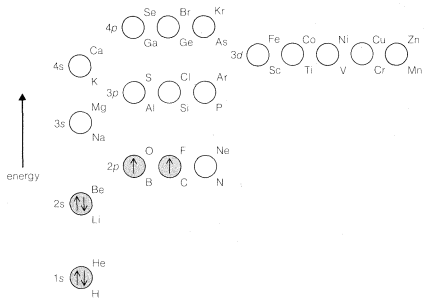
If we assume that all atomic nuclei have orbitals like those of the hydrogen atom, we can see how atoms more complex than hydrogen can be built up by adding electrons to the orbitals in accord with the Pauli exclusion principle. The lowest-energy states will be those in which the electrons are added to the lowest-energy orbitals. For example, the electronic configuration of the lowest-energy state of a carbon atom is shown in Figure 6-4, which also shows the relative energies of the \(1s\) through \(4p\) atomic orbitals. The orbitals of lowest energy are populated with the proper number of electrons to balance the nuclear charge of \(+6\) for carbon and to preserve the Pauli condition of no more than two paired electrons per orbital. However, the two highest-energy electrons are put into different \(2p\) orbitals with unpaired spins in accordance with Hund's rule. The rationale of Hund's rule depends on the fact that electrons come closer together. Now, suppose there are two electrons that can go into two different orbitals of the same energy (so-called degenerate orbitals). Hund's rule tells us that the repulsion energy between these electrons will be less if they have unpaired spins (\(\uparrow \uparrow\)). Why is this so? Because if they have unpaired

Figure 6-4: Diagram showing the most stable electronic configuration, \(\left( 1s \right)^2 \left( 2s \right)^2 \left( 2p_x \right)^1 \left( 2p_y \right)^1\), of a carbon atom. Addition of more electrons in accord with Hund's rule gives the electronic configuration of the other atoms indicated by the atomic symbols.

spins they cannot be in the same orbital at the same time. Therefore they will not be able to approach each other as closely as they would if they could be in the same orbital at the same time. For this reason the electronic configuration

Two circles each with an arrow pointing up inside.

is expected to be more stable than the configuration

Left: Two circles with arrows inside. Left circle has arrow pointing up and right circle has arrow pointing down. OR right: two circles. Left circle has two arrows; one pointing up and one pointing down. Left circle is empty.

if both orbitals have the same energy.

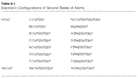
States such as the one shown in Figure 6-4 for carbon are built up through the following steps. Helium has two paired electrons in the \(1s\) orbital; its configuration can be written as \(\left( 1s \right)^2\), the superscript outside the parentheses denoting two paired electrons in the \(1s\) orbital. For lithium, we expect \(Li \: \left( 1s \right)^2 \left( 2s \right)^1\) to be the ground state, in which the \(1s\) electrons must be paired according to the exclusion principle. Continuing in this way, we can derive the electronic configurations for the elements in the first three rows of the periodic table, as shown in Table 6-1. These configurations conform to the

Table of electronic configurations of ground states of atoms — Figure 6-4.

\(^1\)The index number refers to the principal quantum number and corresponds to the "\(K\) shell" designation often used for the electron of the normal hydrogen atom. The principal quantum number 2 corresponds to the \(L\) shell, 2 to the \(M\) shell, and so on. The notation \(s\) (also \(p\), \(d\), \(f\) to come later) has been carried over from the early days of atomic spectroscopy and was derived from descriptions of spectroscopic lines as "sharp", "principal", "diffuse", and "fundamental," which once were used to identify transitions from particular atomic states.

Contributors and Attributions

John D. Robert and Marjorie C. Caserio (1977) Basic Principles of Organic Chemistry, second edition. W. A. Benjamin, Inc. , Menlo Park, CA. ISBN 0-8053-8329-8. This content is copyrighted under the following conditions, "You are granted permission for individual, educational, research and non-commercial reproduction, distribution, display and performance of this work in any format."