1.8: N-dimensional cyclic systems

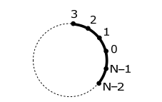
This lecture will provide a derivation of the LCAO eigenfunctions and eigenvalues of N total number of orbitals in a cyclic arrangement. The problem is illustrated below:

There are two derivations to this problem.

Polynomial Derivation

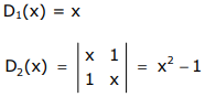
The Hückel determinant is given by,

\[D_{N}(x)=\left|\begin{array}{ccccccccc}
x & 1 & & & & & & & \\
1 & x & 1 & & & & & & \\
& 1 & x & \ddots & & & & & \\
& & 1 & \ddots & \ddots & & & & \\
& & & \ddots & \ddots & \ddots & & & \\
& & & & \ddots & \ddots & \ddots & & \\
& & & & & \ddots & \ddots & 1 & \\
& & & & & & \ddots & x & 1 \\
& & & & & & 1 & x
\end{array}\right|=0\]

where

\[ x=\frac{\alpha-E}{\beta}\]

From a Laplace expansion one finds,

\[D_N(x)=x D_{n-1}(x)-D_{N-2}(x)\]

Where

\[
\begin{array}{l}
D_1(x)=x \\
D_2(x)=\left|\begin{array}{ll}
x & 1 \\
1 & x
\end{array}\right|=x^2-1
\end{array}
\notag \]

 

With these parameters defined, the polynomial form of D_N(x) for any value of N can be obtained,

\[
\begin{array}{c}
D_3(x)=x D_2(x)-D_1(x)=x\left(x^2-1\right)-x=x\left(x^2-2\right) \\
D_4(x)=x D_3(x)-D_2(x)=x^2\left(x^2-2\right)-\left(x^2-1\right)
\end{array}
\notag \]

\[ \vdots \nonumber \]

and so on

The expansion of DN(x) has as its solution,

\[ x={-2}\cos \dfrac{2\pi}{N}j (j= 0, 1, 2, 3...N-1) \nonumber \]

and substituting for x,

\[ E = \alpha + 2\beta\cos \dfrac{2\pi}{N}j (j= 0, 1, 2, 3...N-1) \nonumber \]

Standing Wave Derivation

An alternative approach to solving this problem is to express the wavefunction directly in an angular coordinate, θ

For a standing wave of λ about the perimeter of a circle of circumference c,

\[ \psi_j = \sin \dfrac{c}{\lambda} \theta \nonumber \]

The solution to the wave function must be single valued ∴ a single solution must be obtained for ψ at every 2nπ or in analytical terms,

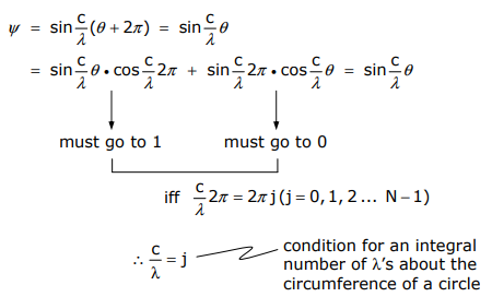
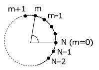
Thus the amplitude of \(ψ_j\) at atom m is, (where c/λ = j and θ = (2π/N)m)

\[ \psi_{j}(m) = \sin{2m\pi}{N}j (j= 0, 1, 2, 3...N-1) \nonumber \]

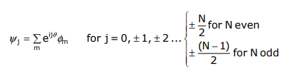
Within the context of the LCAO method, ψ_j may be rewritten as a linear combination in φ_m with coefficients c_jm. Thus the amplitude of ψ_j at m is equivalent to the coefficient of φ_m in the LCAO expansion,

\[ \psi_{j} = \displaystyle \sum_{k=1}^N C_{jm\phi m} \]

Where

\[C_{jm} = \sin{2\pi m}{N}j (j= 0, 1, 2, 3...N-1) \nonumber \]

The energy of each MO, ψ_j, may be determined from a solution of Schrödinger’s equation,

\[
\begin{array}{l}
\mathrm{H} \psi_j=\mathrm{E}_j \psi_j \\
\left.\left|\mathrm{H}-\mathrm{E}_{\mathrm{j}}\right| \psi_j\right\rangle=0 \\
\left.\left|\mathrm{H}-\mathrm{E}_j\right| \sum_m^{\mathrm{N}} \mathrm{c}_{j m} \phi_m\right\rangle=0
\end{array}
\notag \]

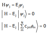
The energy of the φ_m orbital is obtained by left–multiplying by φ_m,

\[\left\langle\phi_m\left|H-E_j\right| \sum_m^N c_{j m} \phi_m\right\rangle=0 \notag \]

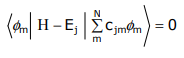
but the Hückel condition is imposed; the only terms that are retained are those involving φ_m, φ_m+1, and φ_m-1. Expanding,

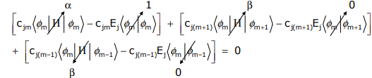
Evaluating the integrals,

\[
\begin{array}{l}
\alpha \mathrm{c}_{j m}-\mathrm{c}_{j m} \mathrm{E}_{\mathrm{j}}+\beta\left\lfloor\mathrm{c}_{\mathrm{j}(\mathrm{m}+1)}+\mathrm{c}_{j(\mathrm{~m}-1)}\right\rfloor=0 \\
\alpha \mathrm{c}_{j m}+\beta\left\lfloor\mathrm{c}_{j(m+1)}+\mathrm{c}_{\mathrm{j}(\mathrm{m}-1)}\right\rfloor=\mathrm{c}_{j m} \mathrm{E}_{\mathrm{j}}
\end{array}
\no tag\]

Substituting for c_jm,

\[ \alpha \sin \dfrac{2\pi m}{N}j + \beta \left( \sin \dfrac{2\pi (m+1)}{N}j + \sin \dfrac{2\pi (m-1)}{N}j \right) = E_{j} \sin \dfrac{2\pi m}{N}j \nonumber \]

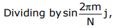
\[ \alpha + \dfrac{ \beta \left( \sin \dfrac{2\pi (m+1)}{N}j + \sin \dfrac{2\pi (m-1)}{N}j \right)}{ \sin \dfrac{2\pi m}{N}j} = E_{j} \nonumber \]

Making the simplifying substitution, \(\kappa=\frac{2 \pi}{N} j\)
\[
\mathrm{E}_{\mathrm{j}}=\alpha+\beta\left(\frac{\sin \kappa \mathrm{m} \cdot \cos \kappa+\sin \kappa \cdot \cos \kappa \mathrm{m}+\sin \kappa \mathrm{m} \cdot \cos \kappa-\sin \kappa \cdot \cos \kappa \mathrm{m}}{\sin \kappa \mathrm{m}}\right)
\notag \]

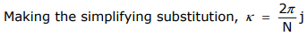
\[ E_{j} = \alpha + 2\beta \cos k \nonumber \]

\[ E_{j} = \alpha + 2\beta \cos \dfrac{2\pi}{N}j (j= 0, 1, 2, 3...N-1) \nonumber \]

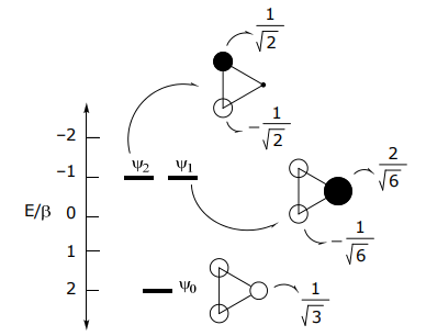
Let’s look at the simplest cyclic system, N = 3

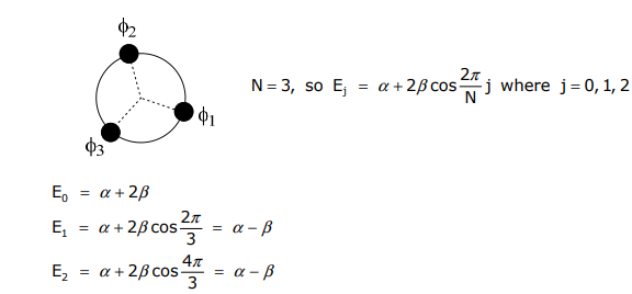
Continuing with our approach (LCAO) and using Ej to solve for the eigenfunction, we find…

\[
\psi_j=\sum_m e^{i j \theta} \phi_m \quad \text { for } j=0, \pm 1, \pm 2 \ldots\left\{\begin{array}{l} 
\pm \frac{N}{2} \text { for } N \text { even } \\
\pm \frac{(N-1)}{2} \text { for } N \text { odd }
\end{array}\right.
\]

Using the general expression for ψj, the eigenfunctions are:

\[ \psi_{0} = e^{i(0)0} \phi_{1} + e^{i(0) \dfrac{2\pi}{3}} \phi_{2} + e^{i(0) \dfrac{4\pi}{3}} \phi_{3} \nonumber \]

\[ \psi_{1} = e^{i(1)0} \phi_{1} + e^{i(1) \dfrac{2\pi}{3}} \phi_{2} + e^{i(1) \dfrac{4\pi}{3}} \phi_{3} \nonumber \]

\[ \psi_{-1} = e^{i(-1)0} \phi_{1} + e^{i(-1) \dfrac{2\pi}{3}} \phi_{2} + e^{i(-1) \dfrac{4\pi}{3}} \phi_{3} \nonumber \]

Obtaining real components of the wavefunctions and normalizing,

\[
\begin{array}{ll}
\psi_{0}=\phi_{1}+\phi_{2}+\phi_{3} \rightarrow & \psi_{0}=\frac{1}{\sqrt{3}}\left(\phi_{1}+\phi_{2}+\phi_{3}\right) \\
\psi_{+1}+\psi_{-1}=2 \phi_{1}-\phi_{2}-\phi_{3} \rightarrow & \psi_{1}=\frac{1}{\sqrt{6}}\left(2 \phi_{1}-\phi_{2}-\phi_{3}\right) \\
\psi_{+1}-\psi_{-1}=\phi_{2}-\phi_{3} \rightarrow & \psi_{2}=\frac{1}{\sqrt{2}}\left(\phi_{2}-\phi_{3}\right)
\end{array}
\]

Summarizing on a MO diagram where α is set equal to 0,