10.1.2: Magnetic Susceptibility

Electronic Structure

The electronic structure of coordination complexes can lead to several different properties that involve different responses to magnetic fields. These properties can vary between related compounds because of differences in electron counts, geometry, or donor strength. As a result, magnetic measurement of these materials can be used as a tool to provide insight into the structure of a coordination complex.

Diamagnetic and paramagnetic compounds are two common categories defined by interaction with a magnetic field. Diamagnetic compounds display a very slight repulsion from magnetic fields. The interaction is quite subtle and requires the proper instrumentation if it is to be observed; it’s not something you would normally notice by waving a magnet in front of a vial of coordination complex. In contrast, paramagnetic compounds display a very slight attraction to magnetic fields. In terms of electronic structure, diamagnetic compounds have all of their electrons in pairs whereas paramagnetic compounds have one or more unpaired electrons. These definitions are not limited to coordination complexes. Atmospheric oxygen, O₂, is a common example of a paramagnetic compound. Atmospheric nitrogen, N₂, is a common example of a diamagnetic compound.

Figure \(\PageIndex{1}\): Valence molecular orbital diagrams of N₂ and O₂ show that N₂ is diamagnetic while O₂ is paramagnetic. (CC-BY-NC; Chris Schaller)

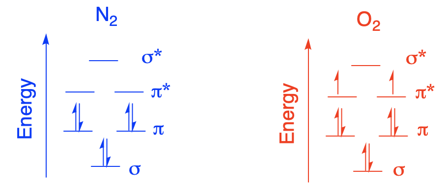
These differences arise because of a quantum mechanical property of electrons and other subatomic particles: spin. Spin does not have a direct macroscopic analogy; physical chemists often urge caution about equating it to a phenomenon on the level at which we observe the universe. However, we do know that spin is related to magnetic phenomena. We can think of an electron as having a magnetic moment. There are two allowed values of this magnetic moment (\(+\frac{1}{2}\) and \(-\frac{1}{2}\)) that differ in orientation; spin is a vector quantity. Normally, there is no preference for one orientation over the other. If a coordination complex has one unpaired electron, and we have a million of those coordination complexes in a very tiny sample, about 500,000 of the unpaired electrons would have spin = \(+\frac{1}{2}\) and about 500,000 of them would have spin = \(-\frac{1}{2}\). The spin of each electron is randomly oriented. As a result, the material would have no net magnetic moment. In the presence of a magnetic field, however, there is a small energy difference between those two spin states. As a result, a majority of the spins adopt the energetically more favorable orientation. Although the material by itself has no net magnetic field, one has temporarily been induced by the influence of an external magnetic field. This is what we mean by magnetic susceptibility.

Measuring Magnetic Susceptibility

All diamagnetic compounds have a roughly similar response to a magnetic field; either their electrons are all paired or they are not. Paramagnetic compounds, however, can respond quite differently to a magnetic field, depending on the number of unpaired electrons. The more unpaired electrons there are, the stronger the magnetic susceptibility will be, and so the stronger the attraction between the compound and the magnetic field. For this reason, measuring the strength of attraction of a compound for a magnetic field can reveal the number of unpaired electrons in the compound. This relationship is most straightforward for complexes of first row transition metals (\(3d\) metals), becoming a little more complicated for the \(4d\) and \(5d\) series.

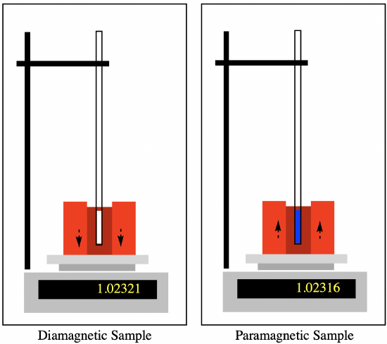
A Guoy balance is probably the simplest example of a method for determining the presence of unpaired electrons in a coordination complex.¹ It uses a balance, a sample holder and a magnet. Essentially, the magnet is weighed in the presence and absence of the sample. The discrepancy between the two measurements arises because of the interaction of the sample with the magnetic field. Any diamagnetic sample causes slight downward repulsion, registering as a heavier weight. A paramagnetic sample suspended between the poles of the magnet causes a slight upward pull on the magnet, which registers as a lighter weight. The more unpaired electrons there are, the greater the induced magnetic moment, and so the lighter the weight becomes.

Figure \(\PageIndex{2}\): Diagram of a Guoy balance. A magnet (red) sits on a balance and a sample tube is placed in the center cavity of the magnet. (CC-BY-NC; Chris Schaller)

From that measurement, we can extract a parameter that we normally refer to as the effective magnetic moment of the material, \(\mu_{eff}\). The magnetic moment is expressed in units called Bohr magnetons. A Bohr magneton (BM or \(\mu_{B}\)) is defined as:

\[1 \text{BM} =\frac{e h}{4 \pi m c} \nonumber \]

in which e is the charge on an electron; \(h\) is Planck’s constant; \(m\) is the mass of the electron; \(c\) is the speed of light.

This experimental quantity is fitted to a simple relationship that depends on the number of unpaired electrons. This mathematical model gives a prediction of the “spin-only” magnetic moment. If the magnetic moment arises purely from the number of unpaired electrons without additional complicating factors, the fit to the experimental data is pretty good.

\[\mu_{ eff } \approx \mu_{ so }=g \sqrt{S(S+1)} \nonumber \]

Here, g is the gyromagnetic ratio, which is a proportionality constant between the angular momentum of the electron and the magnetic moment. It has a value of 2.00023, or approximately 2.0. The term \(\sqrt{S(S+1)}\) is the value of the angular momentum, which depends on the number of unpaired electrons; S is the absolute value of the sum of the individual spins of the valence electrons. Of course, the spins would cancel out in electrons that were paired, because one would have \(m_s = \frac{1}{2}\) and the other would have \(m_s = -\frac{1}{2}\). For unpaired electrons, Hund’s rule states that they would have parallel spins; for example, two unpaired electrons gives \(S=1\).

\[\begin{array}{|c|c|c|} \hline
\text{Number of} & \text{Maximum total} & \text{Spin-only magnetic moment, } \\
\text{unpaired electrons, } n & \text{spin, S} & \mu_{so} (BM) \\ \hline
1 & \frac{1}{2} & 1.73 \\
2 & 1 & 2.83 \\
3 & \frac{3}{2} & 3.87 \\
4 & 2 & 4.90 \\
5 & \frac{5}{2} & 5.92\\ \hline
\end{array} \nonumber \]

The table above shows how the magnetic moment changes with the number of unpaired electrons. The maximum number of unpaired electrons given is five, because for a transition metal a sixth electron would have to pair up in a previously occupied orbital. In f-block elements, there could be seven unpaired electrons before pairing occurs because there are seven f orbitals rather than just five d orbitals.

Note that the expression for spin-only magnetic moment is sometimes written in an alternative way, based directly on the number of unpaired electrons, \(n\), rather than \(S\).

\[\mu_{ eff } \approx \mu_{ so }=\sqrt{n(n+2)} \nonumber \]

There is an additional approximation in these cases, based on how the values of the spin-only magnetic moment correlate with the number of unpaired electrons. If we always round the value of \(\mu_{so}\), then it is one greater than the number of unpaired electrons. Thus, \(\mu_{so} \approx n + 1\), provided of course that there are any unpaired electrons at all; the relationship doesn’t hold if n = 0 because then \(\mu_{so}=0\), not 1.

In reality, observed magnetic moments are slightly different than spin-only magnetic moments. In some cases, the observed magnetic moment is smaller than expected, but those cases are more complicated and we won’t consider them here. Very often, the observed magnetic moments are larger than predicted because orbital angular momentum also plays a role in determining the magnitude of the overall magnetic moment. We may use a modified expression that takes this part into account.

\[\mu_{ eff } \approx \mu_{ s + L }=g \sqrt{S(S+1)+\frac{1}{4} L(L+1)} \nonumber \]

Just as S is the absolute value of the sum of the spin quantum numbers in the ion, \(m_s\), L is the absolute value of the sum of the orbital quantum numbers, \(m_l\). There are five d orbitals, with \(m_l= 2, 1, 0, -1, -2\), and the value of L has to be maximized according to Hund’s rule. That means the value of L can be 3, 2, or 0.

As an example, suppose we have a \(\ce{Co^2+}\) ion. \(\ce{Co^2+}\) ion has a \(d^7\) configuration. It has five \(d\) orbitals, so four of these electrons are paired, leaving only three unpaired electrons with parallel spins, so \(S = 3/2\). In order to maximize the orbital quantum number, \(L\), two electrons will be in an orbital with \(m_l= 2\), two electrons will be in an orbital with \(m_l=1\), and one electron will be in each orbital with \(m_l\) = 0, -1, and -2. When we take the sum, we find \( L = 2 + 2 + 1 + 1 + 0 -1 -2 = 3\). That gives us:

\[\mu_{ s + L }=g \sqrt{3 / 2(3 / 2+1)+\frac{1}{4} 3(3+1)}=5.20 \nonumber \]

In comparison, \(m_{so} = 3.87\) in this case. Observed values of \(\mu_{eff}\) vary between different Co²⁺ complexes but are generally in the range 4.1 – 5.2 BM.² The orbital contribution is often smaller than expected, so magnetic susceptibilities frequently fall somewhere between \(\mu_{so}\) and \(\mu_{S+L}\).

The use of a simple Guoy balance is an historically important method of determining magnetic susceptibility, and it is sometimes used in undergraduate laboratory experiments. Other methods are frequently used to measure magnetic susceptibility in the research laboratory. A magnetic susceptibility balance operates on a similar principle to the one behind the Guoy balance. A sample is placed within the poles of an electromagnet, causing the electromagnet to move very slightly. The current in the electromagnet is adjusted, changing its magnetic field, until the magnet comes back to its initial position. The magnitude of the current adjustment is proportional to the magnetic susceptibility of the sample.

Figure \(\PageIndex{3}\): The Evans Method uses chemical shifts (from NMR) to measure magnetic susceptibility. Left: A capillary tube containing sample and a reference analyte is bathed in a larger tube containing reference analyte solution. Right: The NMR signal of a reference analyte (red) is shifted when that analyte is mixed with a paramagnetic sample (blue). (CC-BY-NC; Chris Schaller)

A superconducting quantum interference device (SQUID) uses a superconducting loop in an external magnetic field to measure magnetic susceptibility of a sample.³ The sample is mechanically moved though the superconducting loop, inducing a change in current and magnetic field that are proportional to the magnetic susceptibility of the sample. Commercially produced SQUID magnetometers often have variable temperature controls, allowing magnetic susceptibility to be measured across a range of temperatures.

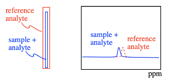
The Evans NMR method is quite common because of the widespread availability of high-field NMR spectrometers in research labs. A capillary containing the paramagnetic sample and a reference analyte is placed in an NMR tube containing the same reference analyte but without the paramagnetic sample. The analyte in the presence of the paramagnetic material will experience a local, induced magnetic field owing to the effect of the superconducting magnet of the NMR instrument on the paramagnetic sample. Its NMR signals will shift as a result. The NMR signal of the analyte outside the capillary will undergo no such shift, and the difference in the two signals is an indicator of the magnetic susceptibility of the sample.

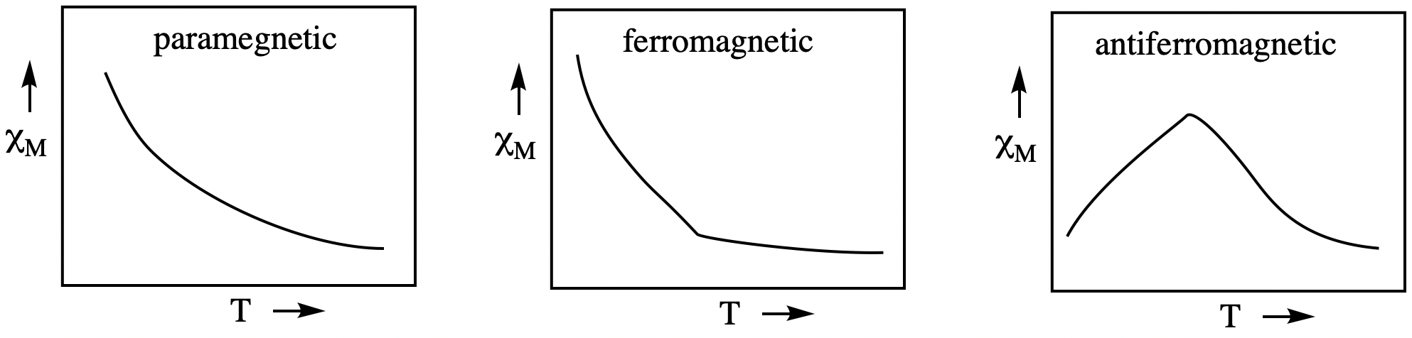
There are other types of magnetic behavior in addition to diamagnetism and paramagnetism. Ferromagnetic materials have long-range order with spins oriented parallel to each other, even in the absence of an external magnetic field. Common, permanent magnets are made from ferromagnetic materials. Antiferromagnetic materials also have long-range order, but the magnetic moments are arranged in opposing pairs. These three different magnetic behaviors are diagnosed by the temperature dependence of the magnetic susceptibility. Paramagnetic materials display magnetic susceptibility (\(\chi_M\), related to \(\mu_{eff}\)_) that increases with the inverse of temperature. Ferromagnetic materials have a critical temperature below which magnetic susceptibility rapidly rises. Antiferromagnetic materials have a critical temperature below which magnetic susceptibility rapidly falls. However, these behaviors are largely beyond the scope of the current discussion.

Figure \(\PageIndex{4}\): Magnetic behavior depends on temperature. Shown are plots of magnetic behaviour in terms of magnetic susceptibility \(\chi_M\) versus temperature (T). (CC-BY-NC; Chris Schaller)

Problems

Exercise \(\PageIndex{1}\)

Show that, given g = 2.0, then \(g \sqrt{S(S+1)}=\sqrt{n(n+2)}\).

Answer

\[\begin{aligned}
\mu_{ so } &=g \sqrt{S(S+1)} \\
&=2 \sqrt{S(S+1)} \\
&=\sqrt{4 S(S+1)} \\
&=\sqrt{2 S(2 S+2)} \end{aligned} \nonumber \]

but \(S=n(1 / 2)\) or \(n=2 S\) then

\[\mu_{ so }=\sqrt{n(n+2)} \nonumber \]

Exercise \(\PageIndex{2}\)

Calculate the value of \(\mu_{so}\) in the following cases:

a) V⁴⁺ b) Cr²⁺ c) Ni²⁺ d) Co³⁺ e) Mn²⁺ f) Fe²⁺

Answer

a) \(V ^{4+} \text{ is } d ^{1} ; n=1 ; \sqrt{n(n+2)}=1.73\)
b) \(Cr ^{2+} \text{ is } d ^{4} ; n=4 ; \sqrt{n(n+2)}=4.90\)
c) \(Ni ^{2+} \text{ is } d ^{8} ; n=2 ; \sqrt{n(n+2)}=2.83\)
d) \(Co ^{3+} \text{ is } d ^{6} ; n=0 ; \sqrt{n(n+2)}=0\)
e) \(Mn ^{2+} \text{ is } d ^{5} ; n=5 ; \sqrt{n(n+2)}=5.92\)
f) \(Fe ^{2+} \text{ is } d ^{6} ; n=4 ; \sqrt{n(n+2)}=4.90\)
g) \(Cr ^{3+} \text{ is } d ^{3} ; n=3 ; \sqrt{n(n+2)}=3.87\)
h) \(V ^{3+} \text{ is } d ^{2} ; n=2 ; \sqrt{n(n+2)}=2.83\)

Exercise \(\PageIndex{3}\)

Calculate the value of \(\mu_{eff}\) in the following cases:

a) V⁴⁺ b) Cr²⁺ c) Ni²⁺ d) Co³⁺ e) Mn²⁺ f) Fe²⁺

g) Cr³⁺ h) V³⁺

Answer

a) \(V ^{4+}\text{ is } d ^{1} ; S=1 / 2 ; L=2 ; \mu_{ s + L }=g \sqrt{1 / 2(1 / 2+1)+\frac{1}{4} 2(2+1)}=3.00\)
b) \(Cr ^{2+}\text{ is } d ^{4} ; S=2 ; L=2+1+0-1=2 ; \mu_{ s + L }=g \sqrt{2(2+1)+\frac{1}{4} 2(2+1)}=5.48\)
c) \(Ni ^{2+}\text{ is } d ^{8} ; S=1 ; L=2+2+1+1+0+0-1-2=3 ; \mu_{ s + L }=g \sqrt{1(1+1)+\frac{1}{4} 3(3+1)}=2.24\)
d) \(Co ^{3+}\text{ is } d ^{6} ; S=2 ; L=2+2+1+0-1-2=2 ; \mu_{ s + L }=g \sqrt{(2+1)+\frac{1}{4} 2(2+1)}=5.48\)
e) \(Mn ^{2+}\text{ is } d ^{5} ; S=5 / 2 ; L=2+1+0-1-2=0 ; \mu_{ s + L }=g \sqrt{5 / 2(5 / 2+1)+\frac{1}{4} 0(0+1)}=5.92\)
f) \(Fe ^{2+}\text{ is } d ^{6} ; S=2 ; L=2+2+1+0-1-2=2 ; \mu_{ s + L }=g \sqrt{2(2+1)+\frac{1}{4} 2(2+1)}=5.48\)
g) \(Cr ^{3+}\text{ is } d ^{3} ; S=3 / 2 ; L=2+1+0=3 ; \mu_{ s + L }=g \sqrt{3 / 2(3 / 2+1)+\frac{1}{4} 3(3+1)}=5.20\)
h) \(V ^{3+}\text{ is } d ^{2} ; S=1 ; L=2+1=3 ; \mu_{ s + L }=g \sqrt{1(1+1)+\frac{1}{4} 3(3+1)}=2.24\)

References

1. Lancashire, R. J. Magnetic Susceptibility https://chem.libretexts.org/Bookshelves/Inorganic_Chemistry/Map%3A_Inorganic_Chemistry_(Housecroft)/04%3A_Experimental_techniques/4.14%3A_Magnetism/Magnetic_Susceptibility_Measurements (accessed Jun 27, 2021).
2. Cotton, F.A.; Wilkinson, G. Advanced Inorganic Chemistry, 4^th Ed. John Wiley & Sons: New York, 1980, p 628.
3. Raja, P. M. V.; Barron, A. R. Magnetism https://chem.libretexts.org/@go/page/55872 (accessed Jun 27, 2021).