1.12: Octahedral ML₆ Sigma Complexes

An octahedral complex comprises a central metal ion and six terminal ligands. If the ligands are exclusively σ-donors, then the basis set for the ligands is defined as follows,

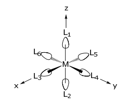
Ligands that move upon the application of an operation, R, cannot contribute to the diagonal matrix element of the representation. Since the σ bond is along the internuclear axis that connects the ligand and metal, the transformation properties of the ligand are correspondent with that of the M–L σ bond. Moreover, a σ bond has no phase change within the internuclear axis, hence the bond can only transform into itself (+1) or into another ligand (0).

\begin{array}{c|cccccccccc}
\mathrm{O}_{\mathrm{h}} & \mathrm{E} & \mathrm{8C}_{3} & 6 \mathrm{C}_{2} & 6 \mathrm{C}_{4} & 3 \mathrm{C}_{2}\left(=\mathrm{C}_{4}{ }^{2}\right) & \mathrm{i} & 6 \mathrm{~S}_{4} & 8 \mathrm{~S}_{6} & 3 \sigma_{\mathrm{h}} & 6 \sigma_{\mathrm{d}} \\
\hline \Gamma_{\mathrm{L} \sigma} & 6 & 0 & 0 & 2 & 2 & 0 & 0 & 0 & 4 & 2
\end{array}

\[\Gamma_{\mathrm{L} \sigma}=\mathrm{a}_{1 \mathrm{~g}}+\mathrm{t}_{1 \mathrm{u}}+\mathrm{e}_{\mathrm{g}}\]

Need now to determine the SALCs of the Lσ basis set. Three different methods will deliver the SALCs.

Method 1

As we have done previously, the SALCs of Lσ may be determined using the projection operator. Note that the ligand mixing in O_h is retained in the pure rotational subgroup, O. Can thus drop from O_h → O, thereby saving 24 operations.

The A₁ irreducible representation is totally symmetric. Hence the projection is simply the sum of the above ligand transformations.

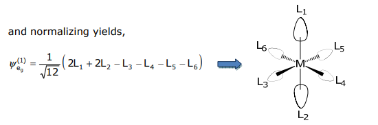
P^A₁(L1) ~ 4(L1 + L2 + L3 + L4 + L5 + L6)

and normalizing yields,

\(
\psi_{a_{19}}=\frac{1}{\sqrt{6}}\left(\mathrm{~L}_{1}+\mathrm{L}_{2}+\mathrm{L}_{3}+\mathrm{L}_{4}+\mathrm{L}_{5}+\mathrm{L}_{6}\right) \)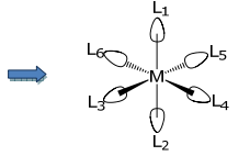
The application of the projection operator for the E irreducible representation furnishes the E_g SALCs.

\( \begin{aligned}
P^{E}\left(L_{1}\right) & \rightarrow\left(2 L_{1}-L_{3}-L_{4}-L_{4}-L_{5}-L_{6}-L_{5}-L_{6}-L_{3}+2 L_{1}+2 L_{2}+2 L_{2}\right) \\
& \rightarrow\left(4 L_{1}+4 L_{2}-2 L_{3}-2 L_{4}-2 L_{5}-2 L_{6}\right)
\end{aligned} \)

But E_g is a doubly degenerate representation, and therefore there is a another SALC. As is obvious from above, the projection operator only yields one of the two SALCs. How do we obtain the other?

Method 2

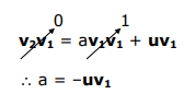
The Schmidt orthogonalization procedure can extract SALCs from a nonorthogonal linear combination of an appropriate basis. Suppose we have a SALC, v₁, then there exists a v₂ that meets the following condition,

v₂ = av₁ + u

where u is the non-orthogonal linear combination. Multiplying the above equation by v₁ gives,

What is the nature of u? Consider using the projection operator on L₃ instead of L₁,

\[\mathrm{P}^{\mathrm{e}_{9}}\left(\mathrm{~L}_{3}\right)=\frac{1}{\sqrt{12}}\left(2 \mathrm{~L}_{3}+2 \mathrm{~L}_{5}-\mathrm{L}_{1}-\mathrm{L}_{2}-\mathrm{L}_{4}-\mathrm{L}_{6}\right)\]

Note, this does not yield any new information, i.e., the atomic orbitals on one axis are twice that and out-of-phase from the atomic orbitals in the equatorial plane. However, this new wavefunction is not ψ_eg⁽²⁾ because it is not orthogonal to ψ_eg⁽¹⁾.

Thus the projection must yield a wavefunction that is a linear combination of ψ_eg⁽¹⁾ and ψ_eg⁽²⁾ , i.e., the wavefunction obtained from the projection is a viable u. Applying the Schmidt orthogonalization procedure,

\[\begin{aligned}
a &=-\mathbf{u v}_{1}=-\left\langle\frac{1}{\sqrt{12}}\left(2 L_{3}+2 L_{5}-L_{1}-L_{2}-L_{4}-L_{6}\right) \mid \frac{1}{\sqrt{12}}\left(2 L_{1}+2 L_{2}-L_{3}-L_{4}-L_{5}-L_{6}\right)\right\rangle \\
&=-\frac{1}{12}[-6]=+\frac{1}{2}
\end{aligned}\]

so,

\[\begin{aligned}
\mathbf{v}_{2} &=\frac{1}{2} \frac{1}{\sqrt{12}}\left(2 L_{1}+2 L_{2}-L_{3}-L_{4}-L_{5}-L_{6}\right)+\frac{1}{\sqrt{12}}\left(2 L_{3}+2 L_{5}-L_{1}-L_{2}-L_{4}-L_{6}\right) \\
&=\frac{1}{\sqrt{12}}\left[\left(\frac{3}{2} L_{3}+\frac{3}{2} L_{5}\right)-\left(\frac{3}{2} L_{4}+\frac{3}{2} L_{6}\right)\right] \approx\left(L_{3}+L_{5}\right)-\left(L_{4}+L_{6}\right)
\end{aligned}\]

ψ_eg⁽²⁾ is orthogonal to ψ_eg⁽¹⁾, thus it is the other SALC.

The T_1g SALCs must now be determined. The projection operator yields,

P^T₁(L₁) → (3L₁ – L₂ – L₂ – L₆ – L₅ – L₄ – L₃ + L₁ + L₁ + L₅ + L₃ + L₄ + L₆ – L₁– L₁ – L₂)

P^T₁(L₁) ~ 3(L₁ – L₂)

and normalizing yields,

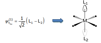
Applying the Schmidt orthogonalization method,

$$
\mathrm{P}^{\mathrm{T}_{1}}\left(\mathrm{~L}_{3}\right) \sim 3\left(\mathrm{~L}_{3}-\mathrm{L}_{5}\right) \rightarrow \psi_{\mathrm{t}_{\mathrm{lu}}}=\frac{1}{\sqrt{2}}\left(\mathrm{~L}_{3}-\mathrm{L}_{5}\right)
\]

This wavefunction is orthogonal to ψ_^t1u⁽¹⁾ , hence it is likely a SALC. Can prove this by t1u applying the Schmidt orthogonalization process and setting this to be u. Solving for a,

$$
\begin{aligned}
a &=-\mathbf{u} \mathbf{v}_{1}=-\left\langle\frac{1}{\sqrt{2}}\left(\mathrm{~L}_{1}-\mathrm{L}_{2}\right) \mid \frac{1}{\sqrt{2}}\left(\mathrm{~L}_{3}-\mathrm{L}_{5}\right)\right\rangle \\
&=-\frac{1}{2}(0)=0
\end{aligned}
\]

and

$$
v_{2}=a v_{1}+u=0 \cdot \frac{1}{\sqrt{2}}\left(L_{1}-L_{2}\right)+\frac{1}{\sqrt{2}}\left(L_{3}-L_{5}\right)
\]

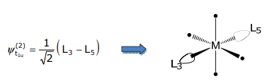
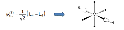
so, as suspected, this is a SALC. And the third SALC of T_1u symmetry is the (L₄,L₆) pair.

Method 3

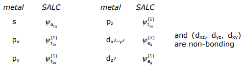
For those SALCs with symmetries that are the same as s, p or d orbitals, may adapt the symmetry of the ligand set to the symmetry of the metal orbitals.

Consider the dz2 orbital, which is more accurately defined as 2z² – x² – y² . Thus the coefficient of the z axis is twice that of x and y and out of phase with x and y. The ligands on the z-axis, L₁ and L₂, should therefore be twice that and of opposite sign to the equatorial ligands, L₃,L₄,L₅,L₆. This leads naturally to,

$$
\begin{aligned}
&\psi_{\mathrm{e}_{9}}^{(1)} \approx 2 \mathrm{~L}_{1}+2 \mathrm{~L}_{2}-\mathrm{L}_{3}-\mathrm{L}_{4}-\mathrm{L}_{5}-\mathrm{L}_{6} \\
&\psi_{\mathrm{e}_{9}}^{(1)}=\frac{1}{\sqrt{12}}\left(2 \mathrm{~L}_{1}+2 \mathrm{~L}_{2}-\mathrm{L}_{3}-\mathrm{L}_{4}-\mathrm{L}_{5}-\mathrm{L}_{6}\right)
\end{aligned}
\]

The other SALC of this degenerate set is given by d_x²–y², which has no coefficient on z, and x and y coefficients that are equal but of opposite sign. By symmetry matching to the orbital,

$$
\begin{aligned}
&\psi_{\mathrm{e}_{9}}^{(2)} \approx \mathrm{L}_{3}-\mathrm{L}_{4}+\mathrm{L}_{5}-\mathrm{L}_{6} \\
&\psi_{\mathrm{e}_{9}}^{(2)}=\frac{1}{2}\left(\mathrm{~L}_{3}-\mathrm{L}_{4}+\mathrm{L}_{5}-\mathrm{L}_{6}\right)
\end{aligned}
\]

The other SALCs follow suit.

The t_2g d-orbital set (i.e. d_xy, d_xz, d_yz) is of incorrect symmetry to interact with the Lσ ligand set and thus is non-bonding. This can be seen from the orbital picture. The Lσ orbitals are directed between the lobes of the t_2g d-orbitals,

Only metal orbitals and SALCs of the same symmetry can overlap. In the case of the octahedral ML₆ σ-complex,

With above considerations of ΔE_ML and S_ML in mind, the MO diagram for M(Lσ)₆ is constructed with Co(NH₃)₆ ³⁺ as the exemplar,

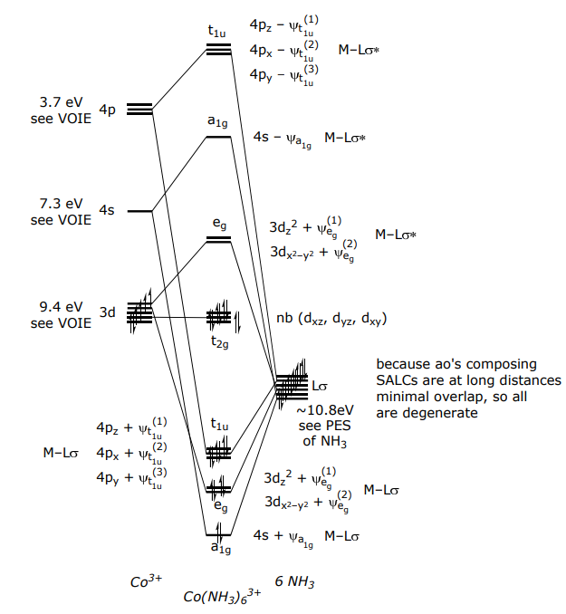
Interaction energies ε_σ and ε_σ* (i.e., the off-diagonal matrix elements, H_ML) are smaller than the difference in energies of the metal and ligand atomic orbitals (i.e., the diagonal matrix elements, H_MM and H_LL), so molecular orbitals stay within their energy “zones”.