1.14: Angular Overlap Method and M-L Diatomics

The Wolfsberg-Hemholtz approximation (Lecture 10) provided the LCAO-MO energy between metal and ligand to be,

$$
\varepsilon_{\sigma}=\frac{\mathrm{E}_{\mathrm{M}}^{2} \mathrm{~S}_{\mathrm{ML}}^{2}}{\Delta \mathrm{E}_{\mathrm{ML}}} \quad \varepsilon_{\sigma^{*}}=\frac{\mathrm{E}_{\mathrm{L}}^{2} \mathrm{~S}_{\mathrm{ML}}^{2}}{\Delta \mathrm{E}_{\mathrm{ML}}}
\]

Note that E_M, E_L and ΔE_ML in the above expressions are constants. Hence, the MO within the Wolfsberg-Hemholtz framework scales directly with the overlap integral, S_ML

$$
\varepsilon_{\sigma}=\frac{\mathrm{E}_{\mathrm{M}}{ }^{2} \mathrm{~S}_{\mathrm{ML}}^{2}}{\Delta \mathrm{E}_{\mathrm{ML}}}=\beta^{\prime} \mathrm{S}_{\mathrm{ML}}^{2} \quad \varepsilon_{\sigma^{*}}=\frac{\mathrm{E}_{\mathrm{L}}^{2} \mathrm{~S}_{\mathrm{ML}}^{2}}{\Delta \mathrm{E}_{\mathrm{ML}}}=\beta \mathrm{S}_{\mathrm{ML}}{ }^{2}
\]

where β and β´are constants. Thus by determining the overlap integral, S_ML, the energies of the MOs may be ascertained relative to the metal and ligand atomic orbitals.

The Angular Overlap Method (AOM), provides a measure of S_ML and hence MO energy levels. In AOM, the overlap integral is also factored into a radial and angular product,

S_ML=S(r)F(θ,Φ)

Analyzing S(r) as a function of the M–L internuclear distance,

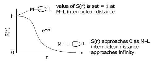
Under the condition of a fixed M-L distance, S(r) is invariant, and therefore the overlap integral, S_ML, will depend only on the angular dependence, i.e., on F(θ,φ).

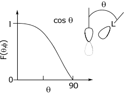
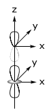
Because the σ orbital is symmetric, the angular dependence, F(θ,φ), of the overlap integral mirrors the angular dependence of the central orbital.

p-orbital

…is defined angularly by a cos θ function. Hence, the angular dependence of a σ orbital as it angularly rotates about a p-orbital reflects the cos θ angular dependence of the p-orbital.

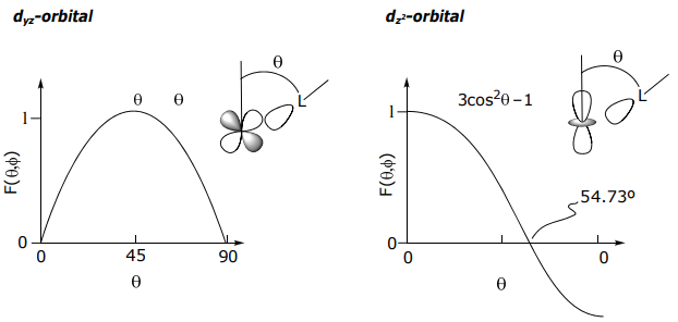
Similarly, the other orbitals take on the angular dependence of the central metal orbital. Hence, for a

ML Diatomic Complexes

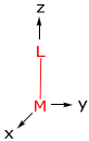
To begin, let’s determine the energy of the d-orbitals for a M-L diatomic defined by the following coordinate system,

There are three types of overlap interactions based on σ, π and δ ligand orbital symmetries. For a σ orbital, the interaction is defined as,

$$
\mathrm{E}\left(\mathrm{d}_{z^{2}}\right)=\mathrm{S}_{\mathrm{ML}}^{2}(\sigma)=\beta \cdot \mathrm{F}_{\sigma}{ }^{2}(\theta, \phi)=\beta \cdot 1=\mathrm{e} \sigma
\]

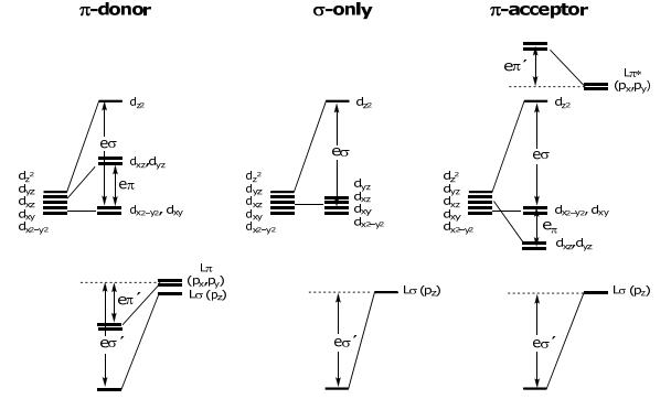
The energy for maximum overlap, at θ = 0 (see above) is set equal to 1. This energy is defined as eσ. The metal orbital bears the antibonding interaction, hence d_z² is destablized by eσ (the corresponding L orbital is stabilized by (β’)2 • 1 = eσ’).

For orbitals of π and δ symmetry, the same holds…maximum overlap is set equal to 1, and the energies are eπ and eδ, respectively.

E(d_yz)=E(d_xz)=S_ML²(π)=eπ E(d_xy)=E(d_x²-y²)=S_ML²(δ)=eδ

As with the σ interaction, the (M-Lπ)* interaction for the d-orbitals is de-stabilizing and the metal-based orbital is destablized by eπ, whereas the Lπ ligands are stabilized by eπ. The same case occurs for a ligand possessing a δ orbital, with the only difference being an energy of stabilization of eδ for the Lδ orbital and the energy of de-stabilization of eδ for the δ metal-based orbitals.

S_ML(δ) is small compared to S_ML(π) or S_ML(σ). Moreover, there are few ligands with δ orbital symmetry (if they exist, the δ symmetry arises from the pπ-systems of organic ligands). For these reasons, the S_ML(δ) overlap integral and associated energy is not included in most AOM treatments.

Returning to the problem at hand, the overall energy level diagrams for a M-L diatomic molecule for the three ligand classes are:

ML₆ Octahedral Complexes

Of course, there is more than 1 ligand in a typical coordination compound. The power of AOM is that the eσ and eπ (and eδ), energies are additive. Thus, the MO energy levels of coordination compounds are determined by simply summing eσ and eπ for each M(d)-L interaction.

Consider a ligand positioned arbitrarily about the metal,

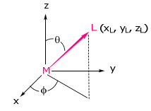
We can imagine placing the ligand on the metal z axis (with x and y axes of M and L also aligned) and then rotate it on the surface of a sphere (thus maintaining M-L distance) to its final coordinate position. Within the reference frame of the ligand,

Note, the coordinate transformation lines up the ligand of interest on the z axis so that the normalized energies, eσ and eπ (and eδ) may be normalized to 1. The transformation matrix for the coordinate transformation is:

$$
\begin{array}{c|cccc}
& \mathbf{z}_{2}{ }^{2} & \mathrm{y}_{2} \mathbf{z}_{2} & \mathrm{x}_{2} z_{2} & \mathrm{x}_{2} \mathrm{y}_{2} & \mathrm{x}_{2}{ }^{2}-\mathrm{y}_{2}{ }^{2} \\
\hline \mathbf{z}^{\mathbf{2}} & \frac{1}{4}(1+3 \cos 2 \theta) & 0 & -\frac{\sqrt{3}}{2} \sin 2 \theta & 0 & \frac{\sqrt{3}}{4}(1-\cos 2 \theta) \\
\mathbf{y z} & \frac{\sqrt{3}}{2} \sin \phi \sin 2 \theta & \cos \phi \cos \theta & \sin \phi \cos 2 \theta & -\cos \phi \sin \theta & -\frac{1}{2} \sin \phi \sin 2 \theta \\
\mathbf{x z} & \frac{\sqrt{3}}{2} \cos \phi \sin 2 \theta & -\sin \phi \cos \theta & \cos \phi \cos 2 \theta & \sin \phi \sin \theta & -\frac{1}{2} \cos \phi \sin 2 \theta \\
\mathbf{x y} & \frac{\sqrt{3}}{4} \sin 2 \phi(1-\cos 2 \theta) & \cos 2 \phi \sin \theta & \frac{1}{2} \sin 2 \phi \sin 2 \theta & \cos 2 \phi \cos \theta & \frac{1}{4} \sin 2 \phi(3+\cos 2 \theta) \\
\mathbf{x}^{2}-\mathbf{y}^{2} & \frac{\sqrt{3}}{4} \cos 2 \phi(1-\cos 2 \theta) & -\sin 2 \phi \sin \theta & \frac{1}{2} \cos 2 \phi \sin 2 \theta & -\sin 2 \phi \cos \theta & \frac{1}{4} \cos 2 \phi(3+\cos 2 \theta)
\end{array}
$$

\(
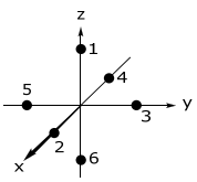
\begin{array}{c|cccccc}
\text { Ligand } & 1 & 2 & 3 & 4 & 5 & 6 \\
\hline \theta & 0 & 90 & 90 & 90 & 90 & 180^{\circ} \\
\phi & 0 & 0 & 90 & 180 & 270 & 0
\end{array}
\)

Consider the overlap of Ligand 2 in the transformed coordinate space; the contribution of the overlap of Ligand 2 with each metal orbital must be considered. This orbital interaction is given by the transformation matrix above. By substituting the θ = 90 and φ = 0 for Ligand 2 into the above transformation matrix, one finds,

for d_z² for L₂

\( \begin{aligned}
\mathrm{d}_{z^{2}} &=\frac{1}{4}(1+3 \cos 2 \theta) d_{z_{2}{ }^{2}}+0 d_{y_{2} z_{2}}-\frac{\sqrt{3}}{2} \sin 2 \theta d_{x_{2} z_{2}}+0 d_{x_{2} y_{2}}+\frac{\sqrt{3}}{4}(1-\cos 2 \theta) d_{x_{2}^{2}-y_{2}^{2}} \\
&=-\frac{1}{2} d_{z_{2}^{2}}+0 d_{y_{2} z_{2}}+0 d_{x_{2} z_{2}}+0 d_{x_{2} y_{2}}+\frac{\sqrt{3}}{2} d_{x_{2}^{2}-y_{2}^{2}}
\end{aligned} \)

Thus the d_z² orbital in the transformed coordinate, d_z2², has a contribution from d_z² and d_x²–y². Recall that energy of the orbital is defined by the square of the overlap integral. Thus the above coefficients are squared to give the energy of the d_z² orbital as a result of its interaction with Ligand 2 to be,

\(
\mathrm{E}\left(\mathrm{d}_{z^{2}}\right)^{\mathrm{L} 2}=\mathrm{S}_{\mathrm{ML}}{ }^{2}(\sigma)=\beta \cdot \mathrm{F}_{\sigma}^{2}(\theta, \phi)=\frac{1}{4} \mathrm{~d}_{\mathrm{z}_{2}{ }^{2}}+\frac{3}{4} \mathrm{~d}_{\mathrm{x}_{2}{ }^{2}-\mathrm{y}_{2}{ }^{2}}=\frac{1}{4} \mathrm{e} \sigma+\frac{3}{4} \mathrm{e} \delta \)

Visually, this result is logical. In the coordinate transformation, a σ ligand residing on the z-axis (of energy eσ) is overlapping with d_z². This is the energy for L1. The normalized energy for L2 is its overlap with the coordinate transformed d_z² 2:

Note, the d_z² orbital is actually 2z² –x² –y² , which is a linear combination of z² –x² and z² –y² . Thus in the coordinate transformed system, L2, as compared to L1, is looking at the x² contribution of the wavefunction to σ bonding. Since it is ½ the electron density of that on the z-axis, it is ¼ the energy (i.e., the square of the coefficient) on the σ-axis, hence ¼ eσ. The δ component of the transformation comes from the 2z² –(x² +y² ) orbital functional form. Thus if L2 has an orbital of δ symmetry, then it will have an energy of ¾ eδ.

The transformation properties of the other d-orbitals, as they pertain to L2 orbital overlap, may be ascertained by completing the transformation matrix for θ = 90 and φ = 0,

$$
\left[\begin{array}{c}
\mathrm{d}_{\mathrm{z}^{2}} \\
\mathrm{~d}_{\mathrm{yz}} \\
\mathrm{d}_{\mathrm{xz}} \\
\mathrm{d}_{\mathrm{xy}} \\
\mathrm{d}_{\mathrm{x}^{2}-y^{2}}
\end{array}\right]=\left[\begin{array}{rrrrr}
-\frac{1}{2} & 0 & 0 & 0 & \frac{\sqrt{3}}{2} \\
0 & 0 & 0 & -1 & 0 \\
0 & 0 & -1 & 0 & 0 \\
0 & 1 & 0 & 0 & 0 \\
\frac{\sqrt{3}}{2} & 0 & 0 & 0 & \frac{1}{2}
\end{array}\right]\left[\begin{array}{c}
\mathrm{d}_{z_{2}{ }^{2}} \\
\mathrm{~d}_{\mathrm{y}_{2} z_{2}} \\
\mathrm{~d}_{\mathrm{x}_{2} \mathrm{z}_{2}} \\
\mathrm{~d}_{\mathrm{x}_{2} y_{2}} \\
\mathrm{~d}_{\mathrm{x}_{2}^{2}-\mathrm{y}_{2}{ }^{2}}
\end{array}\right]
\]

The energy contribution from L2 to the d-orbital levels as defined by AOM is,

\(
\mathrm{E}\left(\mathrm{d}_{\mathrm{yz}}\right)=\mathrm{e} \delta ; \quad \mathrm{E}\left(\mathrm{d}_{\mathrm{xz}}\right)=\mathrm{e} \pi ; \quad \mathrm{E}\left(\mathrm{d}_{\mathrm{xy}}\right)=\mathrm{e} \pi ; \quad \mathrm{E}\left(\mathrm{d}_{x^{2}-y^{2}}\right)=\frac{3}{4} \mathrm{e} \sigma+\frac{1}{4} \mathrm{e} \delta
\)

Until this point, only the L2 ligand has been treated. The overlap of the d-orbitals with the other five ligands also needs to be determined. The elements of the transformation matrices for these ligands are,

\(
L_{1}:\left[\begin{array}{lllll}
1 & 0 & 0 & 0 & 0 \\
0 & 1 & 0 & 0 & 0 \\
0 & 0 & 1 & 0 & 0 \\
0 & 0 & 0 & 1 & 0 \\
0 & 0 & 0 & 0 & 1
\end{array}\right] \quad L_{3}:\left[\begin{array}{rrrrr}
-\frac{1}{2} & 0 & 0 & 0 & \frac{\sqrt{3}}{2} \\
0 & 0 & -1 & 0 & 0 \\
0 & 0 & 0 & 1 & 0 \\
0 & -1 & 0 & 0 & 0 \\
-\frac{\sqrt{3}}{2} & 0 & 0 & 0 & -\frac{1}{2}
\end{array}\right] \quad L_{4}:\left[\begin{array}{ccccc}
-\frac{1}{2} & 0 & 0 & 0 & \frac{\sqrt{3}}{2} \\
0 & 0 & 0 & 1 & 0 \\
0 & 0 & 1 & 0 & 0 \\
0 & 1 & 0 & 0 & 0 \\
\frac{\sqrt{3}}{2} & 0 & 0 & 0 & \frac{1}{2}
\end{array}\right]
\)

\(
\mathrm{L}_{5}:\left[\begin{array}{rrrrr}
-\frac{1}{2} & 0 & 0 & 0 & \frac{\sqrt{3}}{2} \\
0 & 0 & 1 & 0 & 0 \\
0 & 0 & 0 & -1 & 0 \\
0 & -1 & 0 & 0 & 0 \\
-\frac{\sqrt{3}}{2} & 0 & 0 & 0 & -\frac{1}{2}
\end{array}\right] \quad L_{6}:\left[\begin{array}{rrrrr}
1 & 0 & 0 & 0 & 0 \\
0 & -1 & 0 & 0 & 0 \\
0 & 0 & 1 & 0 & 0 \\
0 & 0 & 0 & -1 & 0 \\
0 & 0 & 0 & 0 & 1
\end{array}\right]
\)

Squaring the coefficients for each of the ligands and then summing the total energy of each d-orbital,

$$
\begin{array}{lccccccc}
\hline & \text { L1 } & \text { L2 } & \text { L3 } & \text { L4 } & \text { L5 } & \text { L6 } & \text { E_TOTAL } \\
\hline \mathbf{E}\left(\mathbf{d}_{\mathbf{z}^{2}}\right) & \text { eo } & \frac{1}{4} \mathrm{e} \sigma+\frac{3}{4} \mathrm{e} \delta & \frac{1}{4} \mathrm{e} \sigma+\frac{3}{4} \mathrm{e} \delta & \frac{1}{4} \mathrm{e} \sigma+\frac{3}{4} \mathrm{e} \delta & \frac{1}{4} \mathrm{e} \sigma+\frac{3}{4} \mathrm{e} \delta & \mathrm{e} \sigma & =3 \mathrm{e} \sigma+3 \mathrm{e} \delta \\
\mathbf{E}\left(\mathbf{d}_{\mathrm{yz}}\right) & \mathrm{e} \pi & \mathrm{e} \delta & \mathrm{e} \pi & \mathrm{e} \delta & \mathrm{e} \pi & \mathrm{e} \pi & =4 \mathrm{e} \pi+2 \mathrm{e} \delta \\
\mathbf{E}\left(\mathbf{d}_{\mathrm{xz}}\right) & \mathrm{e} \pi & \mathrm{e} \pi & \mathrm{e} \delta & \mathrm{e} \pi & \mathrm{e} \delta & \mathrm{e} \pi & =4 \mathrm{e} \pi+2 \mathrm{e} \delta \\
\mathbf{E}\left(\mathbf{d}_{\mathrm{xy}}\right) & \mathrm{e} \delta & \mathrm{e} \pi & \mathrm{e} \pi & \mathrm{e} \pi & \mathrm{e} \pi & \mathrm{e} \delta & =4 \mathrm{e} \pi+2 \mathrm{e} \delta \\
\mathbf{E}\left(\mathbf{d}_{\mathbf{x}^{2}-\mathbf{y}^{2}}\right) & \mathrm{e} \delta & \frac{3}{4} \mathrm{e} \sigma+\frac{1}{4} \mathrm{e} \delta & \frac{3}{4} \mathrm{e} \sigma+\frac{1}{4} \mathrm{e} \delta & \frac{3}{4} \mathrm{e} \sigma+\frac{1}{4} \mathrm{e} \delta & \frac{3}{4} \mathrm{e} \sigma+\frac{1}{4} \mathrm{e} \delta & \mathrm{e} \delta & =3 \mathrm{e} \sigma+3 \mathrm{e} \delta \\
\hline
\end{array}
\]

As mentioned above, eδ << e_σ or e_π… thus e_δ may be ignored. The O_h energy level diagram is:

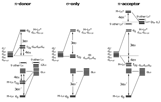
Note the d-orbital splitting is the same result obtained from the crystal field theory (CFT) model taught in freshman chemistry. In fact the energy parametrization scales directly between CFT and AOM

10 Dq = Δ0 = 3eσ – 4eπ