
1.10: General electronic considerations of metal-ligand complexes
- Page ID
- 221678

Metal complexes are Lewis acid-base adducts formed between metal ions (the acid) and ligands (the base).
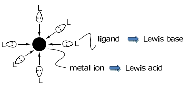
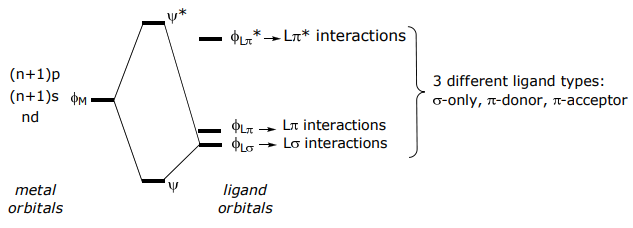
The interaction of the frontier atomic (for single atom ligands) or molecular (for many atom ligands) orbitals of the ligand and metal lead to bond formation,
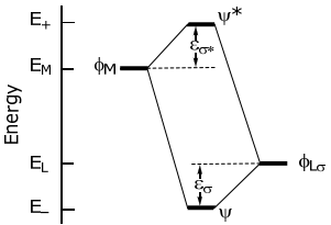
More quantitatively, the interaction energy of stabilization and destabilization, εσ and εσ*, respectively, is defined on the following energy level diagram,
Treating this problem within the LCAO framework comprising metal and ligand orbitals yields,
ψ = cMφM + cLφL
and solving for the Hamiltonian,
$$
\begin{aligned}
&\mathrm{H} \psi=\mathrm{E} \psi \\
&\left.|\mathrm{H}-\mathrm{E}| \psi\rangle=\left|\mathrm{H}-\mathrm{E}_{\mathrm{j}}\right| \mathrm{c}_{\mathrm{M}} \phi_{\mathrm{M}}+\mathrm{c}_{\mathrm{L}} \phi\right\rangle=0
\end{aligned}
\]
Left-multiplying by φM and φL yields the set of linear homogeneous equations,
$$
\begin{aligned}
&c_{M}\left\langle\phi_{M}|H-E| \phi_{M}\right\rangle+c_{L}\left\langle\phi_{M}|H-E| \phi\right\rangle=0 \\
&c_{M}\left\langle\phi_{L}|H-E| \phi_{M}\right\rangle+c_{L}\langle\phi|H-E| \phi\rangle=0
\end{aligned}
\]
which furnishes the secular determinant,
$$
\left|\begin{array}{cc}
\mathrm{H}_{M M}-\mathrm{E} & \mathrm{H}_{M L}-\mathrm{ES}_{M L} \\
\mathrm{H}_{M L}-\mathrm{ES}_{M L} & \mathrm{H}_{L L}-\mathrm{E}
\end{array}\right|=\left|\begin{array}{cc}
\mathrm{E}_{M}-\mathrm{E} & \mathrm{H}_{M L}-\mathrm{ES}_{M L} \\
\mathrm{H}_{M L}-\mathrm{ES}_{M L} & \mathrm{E}_{L}-\mathrm{E}
\end{array}\right|=0
\]

The Wolfsberg-Hemholz approximation provides a value for HML, defined as
HML = SML (EL + EM)
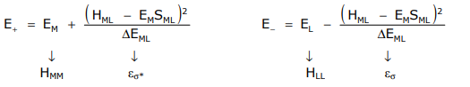
Substituting HML in the above expressions for E+ and E– yields,
$$
\varepsilon_{\sigma}=\frac{E_{M}{ }^{2} S_{M L}{ }^{2}}{\Delta E_{M L}} \quad \varepsilon_{\sigma *}=\frac{E_{L}{ }^{2} S_{M L}{ }^{2}}{\Delta E_{M L}}
\]
The derivation highlights the following general rules for the construction of MO diagrams,
(1) M—L atomic orbital mixing is proportional to the overlap of the metal and ligand orbital, i.e., SML
corollary A: only orbitals of correct symmetry can mix and ∴ give a nonzero interaction energy (i.e. SML ≠ 0)
corollary B: σ interactions typically give rise to larger interaction energies than those resulting from π interactions and π interactions are greater than δ interactions owing to more directional bonding along the series SML(σ) > SML(π) > SML(δ)
(2) M–L atomic orbital mixing is inversely proportional to energy difference of mixing orbitals (i.e. ΔEML).
Another issue of interest for the construction of MOs is,
(3) The order of the EL and EM energy levels almost always is:
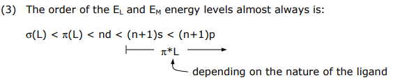
This energy ordering comes directly from Valence Orbital Ionization Energies (VOIE) of metal and main group atoms and PES spectra of molecular ligands.

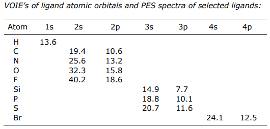
PES energies of ligands are in eVs (note: a VOIE is simply the opposite of the ionization energy)
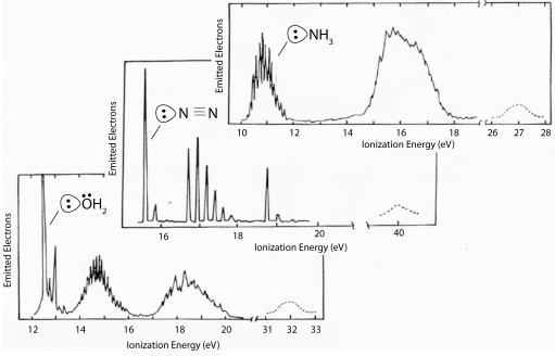
General observations:
(1) The s orbitals are generally too low in energy to participate in bonding (ΔEML(σ) is very large)
(2) Filled p orbitals are the frontier orbitals, and they have VOIEs that place them below the metal orbitals
(3) For molecular ligands, since the frontier orbitals comprise s and p orbitals, here too filled ligand orbitals have energies that are stabilized relative to the metal orbitals