1.3: The Shapes of Molecules (VSEPR Theory) and Orbital Hybridization

The Valence Shell Electron Pair Repulsion (VSEPR) theory is a simple and useful way to predict and rationalize the shapes of molecules. The theory is based on the idea of minimizing the electrostatic repulsion between electron pairs, as first proposed by Sidgwick and Powell in 1940,^[9] then generalized by Gillespie and Nyholm in 1957,^[10] and then broadly applied over the intervening 50+ years.^[11]

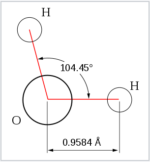
Geometry of the water molecule

To use the VSEPR model, one begins with the Lewis dot picture to determine the number of lone pairs and bonding domains around a central atom. Because VSEPR considers all bonding domains equally (i.e., a single bond, a double bond, and a half bond all count as one electron domain), one can use either an octet or hypervalent structure, provided that the number of lone pairs (which should be the same in both) is calculated correctly. For example, in either the hypervalent or octet structure of the I₃^-ion above, there are three lone pairs on the central I atom and two bonding domains. We then follow these steps to obtain the electronic geometry:

• Determine the number of lone pairs on the central atom in the molecule, and add the number of bonded atoms (a.k.a. bonding domains)
• This number (the steric number) defines the electronic shape of the molecule by minimizing repulsion. For example a steric number of three gives a trigonal planar electronic shape.
• The angles between electron domains are determined primarily by the electronic geometry (e.g., 109.5° for a steric number of 4, which implies that the electronic shape is a tetrahedron)
• These angles are adjusted by the hierarchy of repulsions: (lone pair - lone pair) > (lone pair - bond) > (bond - bond)

The molecular geometry is deduced from the electronic geometry by considering the lone pairs to be present but invisible. The most commonly used methods to determine molecular structure - X-ray diffraction, neutron diffraction, and electron diffraction - have a hard time seeing lone pairs, but they can accurately determine the lengths of bonds between atoms and the bond angles.

The table below gives examples of electronic and molecular shapes for steric numbers between 2 and 9. We are most often concerned with molecules that have steric numbers between 2 and 6.

Bonding electron pairs	Lone pairs	Electron domains (Steric #)	Shape	Ideal bond angle (example's bond angle)	Example	Image
2	0	2	linear	180°	CO2
3	0	3	trigonal planar	120°	BF3
2	1	3	bent	120° (119°)	SO2
4	0	4	tetrahedral	109.5°	CH4
3	1	4	trigonal pyramidal	109.5° (107°)	NH3
2	2	4	bent	109.5° (104.5°)	H2O
5	0	5	trigonal bipyramidal	90°, 120°, 180°	PCl5
4	1	5	seesaw	180°, 120°, 90° (173.1°, 101.6°)	SF4
3	2	5	T-shaped	90°, 180° (87.5°, < 180°)	ClF3
2	3	5	linear	180°	XeF2
6	0	6	octahedral	90°, 180°	SF6
5	1	6	square pyramidal	90° (84.8°), 180°	BrF5
4	2	6	square planar	90°, 180°	XeF4
7	0	7	pentagonal bipyramidal	90°, 72°, 180°	IF7
6	1	7	pentagonal pyramidal	72°, 90°, 144°	XeOF5^−
5	2	7	planar pentagonal	72°, 144°	XeF5^−
8	0	8	square antiprismatic		XeF8^2−
9	0	9	tricapped trigonal prismatic		ReH9^2−

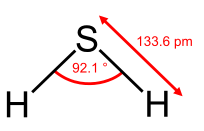
From the Table, we see that some of the molecules shown as examples have bond angles that depart from the ideal electronic geometry. For example, the H-N-H bond angle in ammonia is 107°, and the H-O-H angle in water is 104.5°. We can rationalize this in terms of the last rule above. The lone pair in ammonia repels the electrons in the N-H bonds more than they repel each other. This lone pair repulsion exerts even more steric influence in the case of water, where there are two lone pairs. Similarly, the axial F-S-F angle in the "seesaw" molecule SF₄ is a few degrees less than 180° because of repulsion by the lone pair in the molecule.

Geometrical isomers

For some molecules in the Table, we note that there is more than one possible shape that would satisfy the VSEPR rules. For example, the XeF₂ molecule has a steric number of five and a trigonal bipyramidal geometry. There are three possible stereoisomers: one in which the F atoms occupy axial sites, resulting in linear molecule, one in which the F atoms occupy one equatorial and one axial site (resulting in a 90° bond angle), and one in which the F atoms are both on equatorial sites, with a F-Xe-F bond angle of 120°.

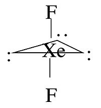
The observed geometry of XeF₂ is linear, which can be rationalized by considering the orbitals that are used to make bonds (or lone pairs) in the axial and equatorial positions. There are four available orbitals, s, p_x, p_y, and p_z. If we choose the z-axis as the axial direction, we can see that the p_x and p_y orbitals lie in the equatorial plane. We assume that the spherical s orbital is shared equally by the five electron domains in the molecule, the two axial bonds share the p_z orbital, and the three equatorial bonds share the p_x and p_y orbitals. We can then calculate the bond orders to axial and equatorial F atoms as follows:

\(axial: \: \frac{1}{5} + \frac{1}{2}p_{z} = 0.7 \: bond (formal \: charge = -0.3)\)

\(equatorial: \: \frac{1}{5}s + \frac{1}{3} p_{x} + \frac{1}{3} p_{y} = 0.867 \:bond (formal \: charge = -0.122)\)

Because fluorine is more electronegative than a lone pair, it prefers the axial site where it will have more negative formal charge. In general, by this reasoning, lone pairs and electropositive ligands such as CH₃ will always prefer the equatorial sites in the trigonal bipyramidal geometry. Electronegative ligands such as F will always go to the axial sites.

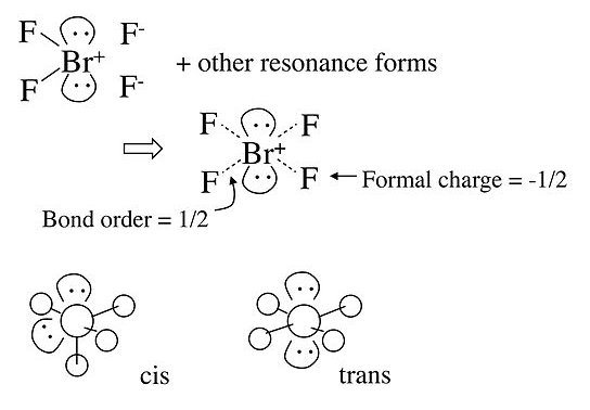
In the case of the BrF₄^- anion, which is isoelectronic with XeF₄ in the Table, the electronic geometry is octahedral and there are two possible isomers in which the two lone pairs are cis or trans to each other. In this case, lone pair - lone pair repulsion dominates and we obtain the trans arrangement of lone pairs, giving a square planar molecular geometry.

Orbital hybridization

The observation of molecules in the various electronic shapes shown above is, at first blush, in conflict with our picture of atomic orbitals. For an atom such as oxygen, we know that the 2s orbital is spherical, and that the 2p_x, 2p_y, and 2p_z orbitals are dumbell-shaped and point along the Cartesian axes. The water molecule contains two hydrogen atoms bound to oxygen not at a 90° angle, but at an angle of 104.5°. Given the relative orientations of the atomic orbitals, how do we arrive at angles between electron domains of 104.5°, 120°, and so on? To understand this we will need to learn a little bit about the quantum mechanics of electrons in atoms and molecules.

The atomic orbitals ψ represent solutions to the Schrödinger wave equation,

\[E \psi = \hat{H} \psi\]

Here E is the energy of an electron in the orbital, and \(\hat{H}\) is the Hamiltonian operator.

By analogy with classical mechanics, the Hamiltonian is commonly expressed as the sum of operators corresponding to the kinetic and potential energies of a system in the form

\[\hat{H} = \hat{T} + \hat{V}\]

where \( \hat{V} = V(\mathbf{r} , t)\) is the potential energy, and

\[ \hat{T} = \frac{\mathbf{\hat{p} \cdot \hat{p}}}{2m} = \frac{\hat{p}^{2}}{2m}= -\frac{\hbar ^{2}}{2m} \nabla ^{2} ,\]

is the kinetic energy operator in which m is the mass of the particle and the momentum operator is:

\[ \hat{p} = -i \mathbf{\hbar} \nabla , \textrm{where} \nabla = \frac{\delta}{\delta x} + \frac{\delta}{\delta y} + \frac{\delta}{\delta z}\]

Here \(\mathbf{\hbar}\) is h/2π, where h is Planck's constant, and the Laplacian operator ∇² is:

\[ \nabla^{2} = \frac{\delta ^{2}}{\delta x^{2}} + \frac{\delta ^{2}}{\delta y^{2}} + \frac{\delta ^{2}}{\delta z^{2}}\]

Although this is not the technical definition of the Hamiltonian in classical mechanics, it is the form it most commonly takes in quantum mechanics. Combining these together yields the familiar form used in the Schrödinger equation:

\[\hat{H} = \hat{T} + \hat{V} = \frac{\mathbf{\hat{p} \cdot \hat{p}}}{2m} + V(\mathbf{r}, t) = - \frac{\mathbf{\hbar ^{2}}}{2m}\nabla^{2} + V(\mathbf{r}, t)\]

For hydrogen-like (one-electron) atoms, the Schrödinger equation can be written as:

\[E \psi = -\frac{\mathbf{\hbar ^ {2}}}{2\mu} \nabla^{2} \psi - \frac{Ze^{2}}{4\pi \epsilon_{0}r} \psi\]

where Z is the nuclear charge, e is the electron charge, and r is the position of the electron. The radial potential term on the right side of the equation is due to the Coulomb interaction, i.e., the electrostatic attraction between the nucleus and the electron, in which ε₀ is the dielectric constant (permittivity of free space) and

\[ \mu = \frac{m_{e}m_{n}}{m_{e} + m_{n}}\]

is the 2-body reduced mass of the nucleus of mass m_n and the electron of mass m_e. To a good approximation, µ ≈ m_e.

Erwin Schrödinger as a young scientist

This is the equation that Erwin Schrödinger famously derived in 1926 to solve for the energies and shapes of the s, p, d, and f atomic orbitals in hydrogen-like atoms. It was a huge conceptual leap for both physics and chemistry because it not only explained the quantized energy levels of the hydrogen atom, but also provided the theoretical basis for the octet rule and the arrangement of elements in the periodic table.

The Schrödinger equation can be used to describe chemical systems that are more complicated than the hydrogen atom (e.g., multi-electron atoms, molecules, infinite crystals, and the dynamics of those systems) if we substitute the appropriate potential energy function V(r,t) into the Hamiltonian. The math becomes more complicated and the equation must be solved numerically in those cases, so for our purposes we will stick with the simplest case of time-invariant, one-electron, hydrogen-like atoms.

Without going into too much detail about the Schrödinger equation, we can point out some of its most important properties:

\[E \psi = -\frac{\mathbf{\hbar ^ {2}}}{2\mu} \nabla^{2} \psi - \frac{Ze^{2}}{4\pi \epsilon_{0}r} \psi\]

• The equation derives from the fact that the total energy (E) is the sum of the kinetic energy (KE) and the potential energy (PE). These three quantities are represented mathematically as operators in the equation.
• On the left side of the equation, the total energy operator (E) is a scalar that is multiplied by the wavefunction ψ. ψ is a function of the spatial coordinates (x,y,z) and is related to the probability that the electron is at that point in space.
• The first term on the right side of the equation represents the kinetic energy (KE). The kinetic energy operator is proportional to ∇² (the Laplacian operator) which takes the second derivative (with respect to three spatial coordinates) of ψ. Thus, the Schrödinger equation is a differential equation.
• The second term on the right side of the equation represents the Coulomb potential (PE), i.e. the attractive energy between the positively charged nucleus and the negatively charged electron.
• The solutions to the Schrödinger equation are a set of energies E (which are scalar quantities) and wavefunctions (a.k.a. atomic orbitals) ψ, which are functions of the spatial coordinates. You will sometimes see the energies referred to as eigenvalues and the orbitals as eigenfunctions, because mathematically the Schrödinger equation is an eigenfunction-eigenvalue equation. Although ψ is a function of the coordinates, E is not. So an electron in a 2p_z orbital has the same total energy E (= PE + KE) no matter where it is in space.
• These E values and their associated wavefunctions ψ are catalogued according to their quantum numbers n, l, and m_l. That is, there are many solutions to the differential equation, and each solution (ψ(xyz) and E) has a unique set of quantum numbers. Some sets of orbitals are degenerate, meaning that they have the same energy (e.g., 2p_x, 2p_y, and 2p_z).
• The solutions ψ(xyz) to the Schrödinger equation (e.g., the 1s, 2s, 2p_x, 2p_y, and 2p_z orbitals) represent probability amplitudes for finding the electron at a particular point (x,y,z) in space. A probability amplitude can have either + or - sign. We typically represent the different signs by shading or by + and - signs on the two lobes of a 2p orbital.
• The square of the probability amplitude, ψ², is always a positive number and represents the probability of finding the electron at a point x,y,z in space. Because the total probability of finding the electron somewhere is 1, the wavefunction must be normalized so that the integral of ψ² over the spatial coordinates (from -∞ to +∞) is 1.
• The solutions to the Schrödinger equation are orthogonal, meaning that the product of any two (integrated over all space) is zero. For example the product of the 2s and 2p_x orbitals, integrated over the spatial coordinates from -∞ to +∞, is zero.

The shapes of the first five atomic orbitals: 1s, 2s, 2px, 2py, and 2pz. The colors denote the sign of the wave function.

Orbital hybridization involves making linear combinations of the atomic orbitals that are solutions to the Schrödinger equation. Mathematically, this is justified by recognizing that the Schrödinger equation is a linear differential equation. As such, any sum of solutions to the Schrödinger equation is also a valid solution. However, we still impose the constraint that our hybrid orbitals must be orthogonal and normalized.

Rules for orbital hybridization:

• Add and subtract atomic orbitals to get hybrid orbitals.
• We get the same number of orbitals out as we put in.
• The energy of a hybrid orbital is the weighted average of the atomic orbitals that make it up.
• The coefficients are determined by the constraints that the hybrid orbitals must be orthogonal and normalized.

For sp hybridization, as in the BeF₂ or CO₂ molecule, we make two linear combinations of the 2s and 2p_z orbitals (assigning z as the axis of the Be-F bond):

\[ \psi_{1} = \frac{1}{\sqrt{2}}(2s) + \frac{1}{\sqrt{2}}(2p_{z})\]

\[ \psi_{2} = \frac{1}{\sqrt{2}}(2s) - \frac{1}{\sqrt{2}}(2p_{z})\]

Here we have simply added and subtracted the 2s and 2pz orbitals; we leave it as an exercise for the interested student to show that both orbitals are normalized (i.e., \(\int \psi_{1}^{2} d\tau = \int \psi_{2}^{2}d\tau = 1\)) and orthogonal (i.e., \( \int \psi_{1} \psi_{2} d \tau =0\)) .

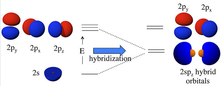
What this means physically is explained in the figure below. By combining the 2s and 2p_z orbitals we have created two new orbitals with large lobes (high electron probability) pointing along the z-axis. These two orbitals are degenerate and have an energy that is halfway between the energy of the 2s and 2p_z orbitals.

Linear combinations of the 2s and 2pz atomic orbitals make two 2spz hybrids. The 2pxand 2py orbitals are unchanged.

For an isolated Be atom, which has two valence electrons, the lowest energy state would have two electrons spin-paired in the 2s orbital. However, these electrons would not be available for bonding. By promoting these electrons to the degenerate 2sp_z hybrid orbitals, they become unpaired and are prepared for bonding to the F atoms in BeF₂. This will occur if the bonding energy (in the promoted state) exceeds the promotion energy. The overall bonding energy, i.e., the energy released by combining a Be atom in its ground state with two F atoms, is the difference between the bonding and promotion energies.

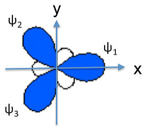
We can similarly construct sp² hybrids (e.g., for the BF₃ molecule or the NO₃^- anion) from one 2s and two 2p atomic orbitals. Taking the plane of the molecule as the xy plane, we obtain three hybrid orbitals at 120° to each other. The three hybrids are:

\[\psi_{1} = \frac{1}{\sqrt{3}}(2s) + \frac{\sqrt{2}}{\sqrt{3}}(2p_{x})\]

\[\psi_{2}= \frac{1}{\sqrt{3}}(2s) - \frac{1}{\sqrt{6}}(2p_{x}) + \frac{1}{\sqrt{2}}(2p_{y})\]

\[\psi_{3}= \frac{1}{\sqrt{3}}(2s) - \frac{1}{\sqrt{6}}(2p_{x}) -\frac{1}{\sqrt{2}}(2p_{y})\]

These orbitals are again degenerate and their energy is the weighted average of the energies of the 2s, 2p_x, and 2p_y atomic orbitals.

Finally, to make a sp³ hybrid, as in CH₄, H₂O, etc., we combine all four atomic orbitals to make four degenerate hybrids:

\[\psi_{1} = \frac{1}{2}(2s + 2p_{x} + 2p_{y} + 2p_{z})\]

\[\psi_{2} = \frac{1}{2}(2s - 2p_{x} - 2p_{y} + 2p_{z})\]

\[\psi_{3} = \frac{1}{2}(2s + 2p_{x} - 2p_{y} - 2p_{z})\]

\[\psi_{4} = \frac{1}{2}(2s - 2p_{x} + 2p_{y} - 2p_{z})\]

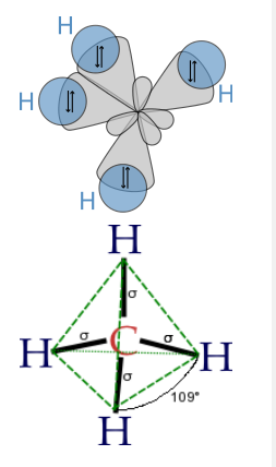
The lobes of the sp³ hybrid orbitals point towards the vertices of a tetrahedron (or alternate corners of a cube), consistent with the tetrahedral bond angle in CH₄ and the nearly tetrahedral angles in NH₃ and H₂O. Similarly, we can show that we can construct the trigonal bipyramidal electronic shape by making sp and sp² hybrids, and the octahedral geometry from three sets of sp hybrids. The picture that emerges from this is that the atomic orbitals can hybridize as required by the shape that best minimizes electron pair repulsions.

Interestingly however, the bond angles in PH₃, H₂S and H₂Se are close to 90°, suggesting that P, S, and Se primarily use their p-orbitals in bonding to H in these molecules. This is consistent with the fact that the energy difference between s and p orbitals stays roughly constant going down the periodic table, but the bond energy decreases as the valence electrons get farther away from the nucleus. In compounds of elements in the 3rd, 4th, and 5th rows of the periodic table, there thus is a decreasing tendency to use s-p orbital hybrids in bonding. For these heavier elements, the bonding energy is not enough to offset the energy needed to promote the s electrons to s-p hybrid orbitals.