2.4: UV-Visible Spectroscopy- Solutions.
- Page ID
- 189757

Exercise 2.1.1
You observe a colored object. Estimate the wavelength of light that was absorbed by the object.
a) 700 nm (just an estimate, but maybe somewhere between 620 and 750 nm)
b) 425 nm c) 540 nm d) 580 nm
Exercise 2.1.2:
a) 590 nm b) 400 nm c) 500 nm d) 300 nm
Exercise 2.1.3
a) 590 nm (strong); that's all b) 400 nm (strong); 600 nm (weak)
c) 500 nm (strong); 350 nm (weak) d) 300 nm (strong); 450 nm (weak)
Exercise 2.1.4
Remember, here we are observing the photons directly, rather than the onew complementary to the absorbed photons.
copper > barium > sodium > calcium > lithium
Exercise 2.2.1:
- 270 nm (strong, MLCT); 500 nm (weak, d-d)
- < 200 nm* (very strong, MLCT); 275 nm (strong, MLCT); 400 nm (weak, d-d) *can't see exactly where because the peak is so tall that we can't see the top
- < 200 nm* (very strong, MLCT); 275 nm (strong, MLCT); 660 nm (weak, d-d)
- < 250 nm (strong, MLCT); 300 nm (strong, MLCT); 620 nm (weak, d-d)
Exercise 2.2.2:
- absorbs blue-green; we see orange-red
- absorbs violet; we see yellow
- absorbs red; we see green
- absorbs orange; we see blue
Exercise 2.2.3:
a) \(A= \varepsilon c l = 14 L g^{-1} cm^{-1} \times 0.025 g L^{-1} \times 1 cm = 0.35\)
a) \(A= \varepsilon c l = 14 L g^{-1} cm^{-1} \times 0.011 g L^{-1} \times 1 cm = 0.15\)
Exercise 2.2.4:
- \(A = \varepsilon c l \: or \: c = \frac{A}{\varepsilon l} = \frac{0.75}{14 L g^{-1} cm^{-1} \times 1cm} = 0.054 g L^{-1}\)
- \(A = \varepsilon c l \: or \: c = \frac{A}{\varepsilon l} = \frac{0.21}{14 L g^{-1} cm^{-1} \times 1cm} = 0.015 g L^{-1}\)
Exercise 2.2.5:
Based on our color wheel it absorbs both yellow and green; we see a mix of violet and red. (KMnO4 is really a deep purple.)
Exercise 2.2.6:
KMnO4 has MW = 158 g mol-1
\[14 \frac{L}{g \: cm} \times 158 \frac{g}{mol} = 2212 \frac{L}{mol \: cm} \nonumber\]
Exercise 2.2.7:
a) \(A = \varepsilon c l = 2200 L mol^{-1} cm^{-1} \times 0.00015 mol L^{-1} \times 1cm = 0.33\)
b) \(A = \varepsilon c l = 2200 L mol^{-1} cm^{-1} \times 0.00009 mol L^{-1} \times 1cm = 0.20\)
Exercise 2.2.8:
- \(A = \varepsilon c l \: or \: c = \frac{A}{\varepsilon l} = \frac {0.47}{2200 L mol^{-1} cm^{-1} \times 1 cm} = 2.1 \times 10^{-4} mol L^{-1}\)
- \(A = \varepsilon c l \: or \: c = \frac{A}{\varepsilon l} = \frac {0.89}{2200 L mol^{-1} cm^{-1} \times 1 cm} = 4.1 \times 10^{-4} mol L^{-1}\)
Exercise 2.3.1:
a) blue b) orange
Exercise 2.3.2:
Add another 30 or 40 nm and you get to 270 or 280 nm.
Exercise 2.3.3:
a) about 250 nm b) about 280 nm
Exercise 2.3.4:
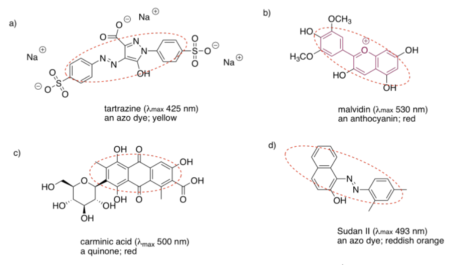
a)
b) yellow
Exercise 2.3.5: