21.7: Molecular Orbitals

In order to explain both the ground state and the excited state involved in an absorption band in the ultraviolet and visible spectra of molecules, it is necessary to look at the electronic structure of molecules in somewhat different terms from the description given in the sections on Chemical Bonding and Further Aspects of Covalent Bonding. In those chapters we treated electrons either as bonding pairs located between two nuclei, or as lone pairs associated with a single nucleus. Such a model of electronic structure is known as the valence-bond model. It is of very little use in explaining molecular spectra because photons are absorbed by the whole molecule, not an individual atom or bond. Thus we need to look upon electrons in a molecule as occupying orbitals which belong to the molecule as a whole. Such orbitals are called molecular orbitals, and this way of looking at molecules is referred to as molecular-orbital (abbreviated MO) theory.

The term molecular orbital is mentioned in the discussion of The Covalent Bond when we described formation of a covalent bond in an H₂ molecule as a result of overlap of two 1s atomic orbitals—one from each H atom. In that section, however, we do not point out that there are two ways in which the 1s electron wave of one H atom can combine with the 1s electron wave of another. One of these involves constructive interference between the two waves and is referred to as positive overlap. This results in a bigger electron wave (and hence more electron density) between the two atomic nuclei. This attracts the positively charged nuclei together, forming a bond as described in "The Covalent Bond". A molecular orbital formed as a result of positive overlap is called a bonding MO.

It is also possible to combine two electron waves so that destructive interference of the waves occurs between the atomic nuclei. This situation is referred to as negative overlap, and it decreases the probability of finding an electron between the nuclei. In the case of two H atoms this results in a planar node of zero electron density halfway between the nuclei. Without a buildup of negative charge between them, the nuclei repel each other and no chemical bond is possible. A molecular orbital formed as a result of negative overlap is called an antibonding MO.

Figure \(\PageIndex{1}\) Energy levels and electron dot-density diagrams for atomic and molecular orbitals associated with hydrogenic 1s wave functions.

If one or more electrons occupy an antibonding MO, the repulsion of the nuclei increases the energy of the molecule, and so such an orbital is higher in energy than a bonding MO. This is shown in Figure \(\PageIndex{1}\). Electron dot-density diagrams for the 1s electron in each of two separate H atoms are shown on the left and right sides of the figure. The horizontal lines show the energy each of these electrons would have. A dot-density diagram for a single electron occupying the bonding MO formed by positive overlap of the two orbitals is shown in the center of the diagram. This is labeled σ_1s. Above it is a dot-density diagram for a single electron occupying the antibonding MO, σ_1s^*. (In general, antibonding MO’s are distinguished from bonding MO’s by adding an * to the label.) The energies of the molecular orbitals are indicated by the horizontal lines in the center of the diagram. The Greek letter σ in the labels for these orbitals refers to the fact that their positive or negative overlap occurs directly between the two atomic nuclei. Like an atomic orbital, each molecular orbital can accommodate two electrons. Thus the lowest energy arrangement for H₂ would place both electrons in the a_1s MO with paired spins. This molecular electron configuration is written (σ_1s)², and it corresponds to a covalent electron-pair bond holding the two H atoms together. If a sample of H₂ is irradiated with ultraviolet light, however, an absorption band is observed between 110 and 170 nm. The energy of such an absorbed photon is enough to raise one electron to the antibonding MO, producing an excited state whose electron configuration is (σ_1s)¹(σ_1s^*)¹. In this excited state the effects of the bonding and the antibonding orbitals exactly cancel each other; there is no overall bond between the two H atoms, and the H₂ molecule dissociates. When the absorption of a photon results in the dissociation of a molecule like this, the phenomenon is called photodissociation. It occurs quite frequently when UV radiation strikes simple molecules.

The molecular-orbital model we have just described can also be used to explain why a molecule of He₂ cannot form. If a molecule of He₂ were able to exist, the four electrons would doubly occupy both the bonding and the antibonding orbitals, giving the electron configuration (σ_1s)²(σ_1s^*)². However, the antibonding electrons would cancel the effect of the bonding electrons, and there would be no resultant buildup of electronic charge between the nuclei and hence no bond. Interestingly enough, an extension of this argument predicts that if He₂ loses an electron to become the He₂⁺ ion, a bond is possible. He₂⁺ would have the structure (σ_1s)²(σ_1s^*)¹ and the single electron in the antibonding orbital would only cancel half the effect of the two electrons in the bonding orbital. This would leave the ion with a “half-bond” joining the two nuclei. The spectrum of He shows bands corresponding to He₂⁺, and from them it can be determined that He₂⁺ has a bond enthalpy of 322 kJ mol^–1.

The molecular-orbital model can easily be extended to other diatomic molecules in which both atoms are identical (homonuclear diatomic molecules). Three general rules are followed. First, only the core orbitals and the valence orbitals of the atoms need be considered. Second, only atomic orbitals whose energies are similar can combine to form molecular orbitals. Third, the number of molecular orbitals obtained is always the same as the number of atomic orbitals from which they were derived.

Applying these rules to diatomic molecules which consist of atoms from the second row of the periodic table, such as N₂, O₂, and F₂, we need to consider the 1s, 2s, 2p_x, 2p_y, and 2p_z atomic orbitals. Since the 1s orbital of each atom differs in energy from the 2s, we can overlap the two 1s orbitals separately from the 2s. This gives a σ_1s and a σ_1s^* MO, as in the case of H₂. Similarly, the 2s orbitals can be combined to give σ_2s and σ_2s^* before we concern ourselves with the higher energy 2p orbitals. There are three 2p orbitals on each atom, and so we expect a total of six molecular orbitals to be derived from them.

Figure \(\PageIndex{2}\) The formation of molecular orbitals from 2p orbitals. In each ease the orbitals interact in both a constructive (+) and a destructive (–) sense to produce a bonding and an antibonding orbital. The 2px and 2py orbitals overlap side by side and produce two π orbitals of equal energy and two π* orbitals, also of equal energy. The end-to-end overlap of the 2px orbitals produces σ and σ* orbitals. (The positions of atomic nuclei are indicated by the intersection of axis lines in each drawing.)

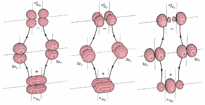
The shapes of these six molecular orbitals are shown by the boundary-surface diagrams in Figure \(\PageIndex{2}\). Two of them are formed by positive and negative overlap of 2p_x orbitals directly between the atomic nuclei. Consequently they are labeled σ_2px and σ_2px*. Two more molecular orbitals are formed by sideways overlap of 2p_x atomic orbitals. These are labeled π_2px and π_2px*, because the molecular orbitals have two parts—one above and one below a nodal plane containing the nuclei. The atomic 2p_y orbitals also overlap sideways to form π_2py and π_2py* molecular orbitals. These are identical to π_2px and π_2px*, except for a 90° rotation around the line connecting the nuclei. Consequently π_2px and π_2py have the same energy, as do π_2px* and π_2py*.

The electron configuration for any homonuclear diatomic molecule containing fewer than 20 electrons can be built up by filling electrons into the molecular orbitals we have just derived, starting with the orbital of lowest energy.

Figure \(\PageIndex{3}\) Relative energies of molecular orbitals for homonuclear diatomic molecules at the time they are being filled. The light lines connect molecular orbitals with the atomic orbitals which they were derived.

The relative energies of the molecular orbitals at the time they are being filled are shown in Figure \(\PageIndex{3}\). Like the energies of atomic orbitals given in Figure 1 from Electron Configurations, these relative molecular-orbital energies vary somewhat from one diatomic molecule to another. In particular the σ_2p orbital is often lower than π_2p. Nevertheless Figure \(\PageIndex{3}\) gives the correct order of filling the orbitals, and we can use it to determine molecular electron configurations.

Example \(\PageIndex{1}\) : Electron Configuration

Find the electronic configuration of the oxygen molecule, O₂.

Solution

Starting with the lowest lying orbitals (σ_1s and σ_1s^*) we add an appropriate number of electrons to successively higher orbitals in accord with the Pauli principle and Hund’s rule. O₂ has 16 electrons, the first 14 of which are easily accommodated in the following way:

\[ ( \sigma_{1s})^2 (\sigma_{1s}^* )^2 ( \sigma_{2s} )^2 (\sigma_{2s}^* )^2 ( \pi_{2p})^4 (\sigma_{2p})^2 \nonumber \]

The remaining two electrons must now be added to the π_2px* orbitals. Since both these orbitals are of equal energy, one electron must be placed in each orbital and the spins must be parallel. The total electronic structure is thus

\[ (\sigma_{1s})^2 (\sigma_{1s}^*)^2 (\sigma_{2s})^2 (\sigma_{2s}^*)^2 ( \pi_{2p})^4 (\sigma_{2p})^2 (\pi_{2px}^*)^1 (\pi_{2py}^*)^1 \nonumber \]

As the previous problem shows, the molecular-orbital model predicts that O₂ has two unpaired electrons. Substances whose atoms, molecules, or ions contain unpaired electrons are weakly attracted into a magnetic field, a property known as paramagnetism. (In a few special cases, such as iron, a much stronger magnetic attraction called ferromagnetism is also obsewed.) Most substances have all their electrons paired. Such materials are weakly repelled by a magnetic field, a property known as diamagnetism. Hence measurement of magnetic properties can tell us whether all electrons are paired or not. O₂, for example, is found to be paramagnetic, an observation which agrees with the electron configuration predicted in Example 21.6. Before the advent of MO theory, however, the paramagnetism was a mystery, since the Lewis diagram predicted that all electrons should be paired.

The molecular-orbital model also allows us to estimate the strengths of bonds in diatomic molecules. We simply count each electron in a bonding orbital as contributing half a bond, while each electron in an antibonding orbital takes away half a bond. Thus if there are B electrons in bonding orbitals and A electrons in antibonding orbitals, the net bond order is given by

\[ \text{ Bond order} = \frac{A-B}{2} \nonumber \]

The larger the bond order, the more strongly the atoms are held together.

Example \(\PageIndex{2}\) : Bond Order

Calculate the bond order for the molecule N₂.

Solution

There are 14 electrons, and so the electron configuration is

\[ ( \sigma_{1s})^2 (\sigma_{1s}^* )^2 ( \sigma_{2s} )^2 (\sigma_{2s}^* )^2 ( \pi_{2p})^4 (\sigma_{2p})^2 \nonumber \]

There are a total of 2 + 2 + 4 + 2 = 10 electrons in bonding MO’s and only 4 in the antibonding orbitals σ_1s^* and σ_2s^*. Thus

\[ \text{ Bond order} = \frac{10-4}{2} = 3 \nonumber \]

The bond orders derived from the molecular-orbital model for stable molecules agree exactly with those predicted by Lewis’ theory. Not only do we find a triple bond for N₂, but we also find a double bond for O₂ and a single bond for F₂. The results of such bond-order calculations are summarized in Table 1.

TABLE \(\PageIndex{1}\) Bond Orders, Bond Enthalpies, and Bond Lengths of Some Diatomic Molecules.

Molecule*	Bond Order	Bond Enthalpy/kJ mol^–1	Bond Length/pm
$$\text{H}^{+}_{2}$$	$$\frac{1}{2}$$	$$256$$	$$106$$
$$\text{H}_2$$		$$432$$	$$74$$
$$\text{He}^{+}_{2}$$	$$\frac{1}{2}$$	$$322$$	$$108$$
$$\text{He}_2$$	$$0$$	$$ \text{Molecule not detected}$$
$$\text{Li}_2$$	$$1$$	$$110$$	$$267$$
$$\text{Be}_2$$	$$0$$	$$ \text{ Molecule not detected}$$
$$\text{B}_2$$	$$1$$	$$274$$	$$159$$
$$\text{C}_2$$	$$2$$	$$603$$	$$124$$
$$\text{N}_2$$	$$3$$	$$942$$	$$110$$
$$\text{O}_2$$	$$2$$	$$494$$	$$121$$
$$\text{F}_2$$	$$1$$	$$139$$	$$142$$
$$\text{Ne}_2$$	$$0$$	$$ \text{Molecule not detected}$$

* Some molecule-ions such as H₂⁺ are included. Except fur the number of electrons involved, the MO theory is applied to them in exactly the same way as to molecules.

Some of the molecules in the table, such as C₂ and B₂, are only stable at high temperatures or only exist transitorily in discharge tubes, and so you are probably not familiar with them. Nevertheless, their spectra can be studied. Also included in the table are values for the bond enthalpies and bond lengths of the various species obtained from their spectra. Note the excellent qualitative agreement with the MO theory. The higher the bond order predicted by the theory, the larger the bond enthalpy and the shorter the bond length.