Techniques for PTV-LVI

Hans-Gerd Janssen, Unilever Research and Development Vlaardingen, the Netherlands

Abstract

The PTV injector is a very flexible injector that can be used for a wide range of different sample introduction techniques. Large volume injection using a PTV can be performed in five different ways.

Level: Advanced

There are five techniques for PTV-LVI:

1. Multiple injection
2. Direct or 'at-once' injection
3. Speed controlled sample introduction
4. Multiple 'at-once' injection
5. PTV on-column injection

The first four of the above mentioned techniques for PTV large volume injection are based on the so-called solvent vent or solvent elimination technique. With these techniques the solvent is evaporated in the liner of the injector and the solvent vapour is discharged via the split exit of the injector. Technique number five is slightly different. PTV on-column large volume injection is largely similar to the standard on-column large volume injection technique described in paragraph 3.2. The only difference is that in the PTV on-column injection the on-column injector is replaced by a PTV injector equipped with a special on-column liner. With this liner the sample can be injected directly into the chromatographic column. PTV on-column large volume sampling has the same advantages and disadvantages as the 'standard' on-column large volume injection technique. From the theoretical point of view it is an excellent technique. For practical reasons, however, one will often try to avoid the use of the method. It is only if none of the other PTV large volume injection methods work, for example because the substances that have to be analysed are extremely volatile or highly unstable, will the PTV on-column technique be the method of choice. For day to day work, this means that the PTV injector is truly a universal interface for large volume injection. With only one injector one can perform various PTV methods for large volume sampling as well as the on-column large volume injection technique. In subsequent paragraphs the various PTV large volume sampling techniques will be discussed in more detail. Particular emphasis will be devoted to the multiple injection technique, 'at-once' injection and speed controlled sampling. As the technique of solvent venting holds a key position in each of the PTV methods for large volume injection, this technique will first be discussed in more detail in a separate paragraph. In all cases it is assumed that the solvent has a lower boiling point than the components of interest. From this it should not be concluded that PTV large volume cannot be used if this is not the case. By carefully exploiting polarity difference or differences in affinity for an adsorbent, also large volumes of samples containing components that are more volatile than the solvent can be successfully analyzed using techniques for PTV large volume sampling. This, however, is outside the scope of the present course. More detailed discussions of the PTV methods can be found in recent literature.

PTV Solvent Elimination

In this section the basic principles of PTV solvent elimination will be briefly summarized. In the first instance it is assumed that only a limited volume of e.g. 1 µl is injected. With the PTV solvent elimination technique the liquid sample is injected into the 'cold' liner of the injector. The word cold here means that the temperature of the injector should be well below the boiling point of the solvent (e.g. at least some 20 to 30 ^oC below the respective solvent boiling point). At the moment of injection the split exit is open. Hence, a relatively high flow of carrier gas is flowing through the injector. A small portion of this gas flows into the column, whereas the vast majority leaves the system via the split exit. Let us take a closer look to the processes occurring in the liner during injection and shortly thereafter.

Let us assume we have an empty liner. When the plunger of the syringe is depressed, a small liquid droplet forms at the tip of the needle. This starts to evaporate, but evaporation is very slow due to the small surface area of the droplet. The droplet grows until it exceeds some critical size and than falls into the liner. It touches the wall and spreads out as a film of liquid. The droplet will not, as some people expect, fall on to the bottom of the injector. This only occurs if an excessive volume is injected (more than can be accommodated by the wall), if the injection is extremely fast or if a liner with a very large inner diameter is used (» 4 mm). After the injection the sample is present as a thin, small liquid film on the wall of the injector. Because the split line is a open, a high flow of gas is flowing across the liquid film that now will be evaporated by the carrier gas. First the solvent will evaporate, as this has the lowest boiling point. The mixture of carrier gas and solvent vapour now passes along the column inlet. A small fraction will enter the column whereas the bulk of gas will be discharged via the split exit. It is only after all of the solvent has evaporated that the other components also start to evaporate. This process is of course slower because of the higher boiling points of these components. Just before this starts to occur the split exit should be closed. In that way the only way components can escape from the liner is via the column. If the injector is heated at this time, all of the solutes will be rapidly transported to the column. To obtain good refocussing here, one would usually work with low initial oven temperatures. It is common practice to choose an oven temperature roughly equal to or slightly above the initial temperature of the PTV injector. The final temperature of the PTV injector should be high enough to yield rapid and quantitative transport of the components of interest within the splitless time selected. If either the final temperature of the PTV is too low or the splitless time is too short, discrimination will be observed for the high boiling sample constituents. It is extremely important that the split exit is closed before the injector is heated. In general it is advisable to wait a few seconds between the moment of closing the split exit and the start of the heating process. In this way flow disturbances that might result from the switching of the split/splitless valve can be damped out.

The PTV solvent injection is schematically depicted in figure 3.2. As can be seen from this figure a solvent elimination injection consists of two steps. In the first step, the actual solvent elimination, the solvent is selectively removed from the injector. In the second step, the splitless transfer, the components left in the liner are transferred to the column in the splitless mode. It is needless to say that both steps have to be optimized carefully. In practice it is generally easier to start optimization with the second step.

2. Temperature and split status during PTV solvent elimination injection

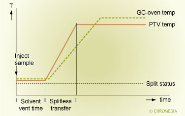
The illustration shows temperature and split status during a PTV solvent elimination injection. Dashed line: split exit open. Solid line: split exit closed.

Large Volume Injection Using the Multiple Injection Method

The easiest method for large volume injection using a PTV injector makes use of the so-called multiple injection mode. This method for large volume injection is schematically depicted in figure 3.3. As the multiple injection mode is seldom used, only a brief description of this technique is given here. An important advantage of the technique is that it is a very easy way to introduce a larger volume (five to ten times the normal injection volume). This gain in sensitivity can be obtained without the need to make any changes to the instrument. It isn’t even necessary to replace the injection port liner.

3. Multiple injection method.

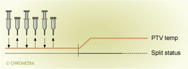
In the multiple injection technique a small volume of sample is injected into the cold injector. This volume should be well below the maximum volume of sample that the liner wall can accommodate. After injection the liquid sample will form a thin film of liquid on the wall of the liner. Depending on the solvent used and the temperature of the PTV injector a typical maximum that can be accommodated by the liner wall is between 5 and 10 µl. If this volume is exceeded, the liquid can not be retained by the liner wall and will be lost via the split exit. During injection the temperature of the injector is low (at least some 30 ^oC below the boiling point of the solvent). One now exploits the mechanism of solvent venting to selectively remove the solvent from the liner. This means that the injection is performed with the split exit open. A high flow of gas is now flowing through the injector. Due to this high flow of gas the solvent evaporates and solvent vapour will be discharged from the injector via the split exit. In one injection only a limited volume of sample can be introduced into the liner because the capacity of the liner to retain the sample is limited. If one now wants to inject a larger volume than can be accommodated by the injector, the process of injection has to be repeated. At a low temperature multiple aliquots of the sample, each of no more than some 5 µl are injected. Between two injections one has to wait to give the solvent of the previous injection sufficient time to evaporate. During this entire process the split exit is kept open. The injection of small sample volumes can be continued until the desired injection volume is reached. After the last injection one waits for a short time to give the solvent from the last injection sufficient time to evaporate. Immediately after this the split exit is closed. Finally, after a few seconds the injector is heated and the components are transferred to the column in the splitless mode.

An important parameter in the multiple injection is the time between two subsequent injections. This time is called the solvent elimination time. The optimum value for this parameter has to be established experimentally. If the time is too short, build up of liquid in the liner will occur and the maximum sample capacity of the liner can be exceeded. This will result in losses of sample. The sample will leave the split exit in the liquid state. In this case all components (both volatile and non-volatiles) will be lost to approximately the same extent. When the time between two injections is too long, serious losses of volatiles will occur. The high boiling components will not be lost. These differences in losses (all components or only volatiles) are the key to the optimization of the multiple injection.

The optimization of a multiple injection can be carried out as follows: Let us assume we want to inject 20 µl of sample as 5 injections of 4 µl. First the PTV conditions are selected. A good initial PTV temperature, when using hexane as the solvent is 30^oC (the boiling point of hexane is 69^oC). For other solvents the PTV temperature has to be adjusted in accordance with the difference of the boiling point of the solvent relative to that of hexane. Apart from the initial temperature of the PTV the final temperature and the splitless time also have to be selected. If the final temperature is too low and/or the splitless time is too short, losses of heavy components (discrimination) can occur. To achieve a rapid evaporation of the solvent it is advantageous to use a split flow that is sufficiently high (>100 mL/min). Split flows as high as 200 to 250 mL/min are more or less standard in the various methods for PTV large volume injection. As a rule of the thumb: The evaporation rate doubles when the split flow is increased by a factor of two. Or expressed as evaporation times: the evaporation time is reduced by a factor of two when the split flow is doubled. When all conditions are selected a first reference chromatogram is recorded. This is done by the analysis of 4 µl of a 5 times or, e.g., 1 µl of a 20 times concentrated sample. The peak areas in this reference chromatogram can be used to calculate the recoveries in the multiple injection of the diluted sample. It is a prerequisite for this method of optimization that the components that are to be analyzed are available in the laboratory. If this is not the case, the optimization can also be carried out using a similar substance or any other substance with a similar boiling point as the component of interest. Because the losses that occur from the injector are almost exclusively based on the vapour pressure of the components, the procedure can also be optimized using a standard solution of a series of normal alkanes in the solvent that is to be used. An additional advantage of using an alkane standard for optimization is that losses of components due to adsorption or thermal degradation can be precluded. Once again, good results in a multiple injection are only obtained if the conditions for splitless transfer of the components to the column (PTV final temperature, heating rate, splitless time) are carefully chosen.

Once the reference chromatogram of the concentrated standard is recorded, the experimental optimization of the solvent elimination time (time between two injections or interval time) can be commenced. To avoid contamination of the carrier gas inlet system and the detector, it is advisable to start the optimization with interval times for which one is sure that it is too long. Under the conditions mentioned above (5 injections of 4 µl each, solvent hexane, PTV temperature 30^oC, split flow 250 mL/min) an interval time of 10 seconds between two subsequent injections is amply sufficient. Under these conditions losses of volatiles will occur. In subsequent experiments the time between two injections can be reduced slowly in order to reduce the losses of volatiles and, eventually, reach conditions where losses are negligible. If the time is reduced too far, one will move from a situation in which only volatiles are lost, to a situation in which all components show less than quantitative recoveries. The optimum is somewhere in between these two times. It is possible that the time between two injections, required to avoid the loss of volatiles, is inpractically short. In this case the solvent elimination can be carried out at a lower temperature or at a lower split flow. In both cases the evaporation proceedes at a lower rate.

In the process of optimizing the time interval between two injections, one can use the fact that too short an time interval gives different problems from too long a time. If, in comparison with the reference chromatogram, all components are lost to some extent then the time is too short. In this instance the samples is lost from the liner in the liquid state. If, on the other hand, only volatile components are lost, the time is too short. Even after a careful optimization of the solvent-elimination time losses of volatile components are difficult if not impossible to avoid. When using hexane as the solvent, components more volatile that roughly normal C₁₄ will be partially lost, despite careful optimization. The best possible situation occurs when the solvent is evaporated at as low a temperature as possible. Also a relatively low split flow (around 100 mL/min) is advantageous for these samples. Losses are minimized if the solvent in the injector is not evaporated to full dryness.

4. Multiple (10)injections of alkane standard (1.5 ppm) in hexane.

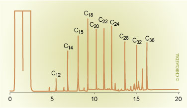
Example of a multiple injection. Sample: alkane standard (1.5 ppm) in hexane. 10 injections of 1.5 µl each. Interval time = 5 seconds.

The illustration shows an example of a chromatogram of a diluted alkane standard recorded using the multiple injection technique. From figure 3 it can be seen that the multiple injection technique, analogous to the solvent vent technique, actually consists of two sucessive steps (solvent elimination and splitless transfer). Each of these two steps has to be carefully optimized. Optimization of the splitless transfer can be performed via an injection of a small volume (e.g. 1µl). The multiple injection method is not really suited for automated routine applications. It is, however, a simple way to increase the injection volume and sensitivity by a factor of up to ten. As no instrumental modifications are required, it is a good method when an increased sensitivity is only required once in a while.

Rapid or 'at-once' injection

The Rapid or 'at-once' injection method for PTV large volume injection bears a close resemblance to the standard solvent vent injection. What is different, however, is that the liner is now filled with a packing material. This can, for example, be glass wool, quartz wool or some other type of material. The main purpose of putting a packing material in the liner is to increase the capacity of the liner to retain the liquid sample. In the 'at-once' large volume injection method the sample is injected rapidly (within a few seconds). After the injection the needle is withdrawn from the injector. The temperature during injection is again well below the boiling point of the solvent. The temperature profile of the injector versus time and the status of the split valve are schematically depicted in figure 5.

Temperature/time profile and split valve status during the direct 'at-once' lvi.

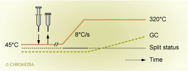
Immediately after the injection the liquid sample will spread out as a thin film of sample over the packing material in the liner. During and immediately after the sample introduction, the split exit of the injector is open and a large flow of carrier gas flows through the injector. The largest part of the gas flow leaves the system via the split exit. Only a small fraction enters the column. Due to the high flow of gas through the liner, the solvent film in the liner starts to evaporate. This evaporation consumes a lot of energy. Therefore, a cold spot is created at the location where the evaporation occurs. In this cold spot, the components present in the sample are well retained. This is not only due to the low temperature, the solutes are also retained by the solvent film present in the cold spot. Despite the rapid and strong cooling that occurs, the process of evaporation in the liner continues. Vapours formed upon evaporation are discharged via the split exit (and to a small extent also via the column). Just before all liquid in the injector is evaporated the split exit is closed and the injector is heated. All components are now transferred to the column in the splitless mode. Figure 6 shows the variation of temperature inside the liner immediately after the injection of a large sample volume. The figure clearly shows the rapid temperature decrease upon injection.

6. Creation of a cold spot in the injector during a rapid injection

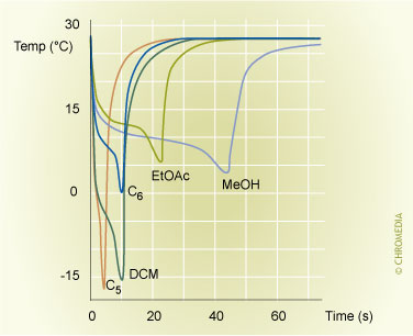
6. Creation of a cold spot in the injector during a rapid injection of a large volume of hexane (100 µl) in a glass wool packed liner. Initial PTV temperature 30^oC. Temperature measured directly below injection point.