Photomultiplier Tubes

In considering the behavior of a photomultiplier tube, a drawing may be helpful.

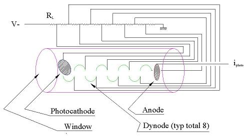
The resistive voltage divider provides potential to each of the electrodes (photocathode, dynodes) except for the anode, which is maintained at virtual common by external circuits. The envelope of the photomultiplier is typically quartz; only wavelengths that can be tranmitted through the window to the photocathode can be detected. The layout shown is for an "end-on" tube. Side-on tubes are also common. For high speed response, there are usually capacitors as well as resistors in the biasing network.

The Photoelectric Effect

When a photon with energy E = hc/λ (h = Planck's constant ~ 6.626×10^-34 Joule S, c = speed of light ~ 2.997×10⁸m s^-1, λ = wavelength, E = energy of a single photon in Joules) strikes a surface, it may be reflected, scattered, or absorbed. If it is absorbed, conservation of energy requires that the energy go somewhere. Some will set up vibrations in the solid lattice -- phonons, or heat. But if the energy of the photon is above the work function of the material (the energy needed to remove an electron from the solid into air or vacuum), the photon has some probability of ejecting such an electron. The quantum efficiency of the photoelectric effect is (number of electrons ejected) / (number of incident photons). It is quite dependent on wavelength, the structure of the material, and temperature. Typically, a photoresponsive surface is maintained at a negative potential so that any electrons that are removed are repelled by the surface from which they've come. Thus, the photoresponsive surface is typically called a photocathode.

Dynodes for Gain

Once an electron is repelled by the photocathode, where will it go? Towards any surface that is more positive. If one has a metal electrode near the photocathode and at a less negative/more positive potential, the electron will head there. If the voltage difference is high enough, the electron will gain enough energy that when it hits the more positive piece of metal (the dynode), it has enough energy to eject more than 1 electron. There is thus an increase in the number of electrons; one photoelectron generates m electrons (m>1) when it collides with a dynode. If there are N dynodes, each at the same voltage more positive than its predecessor, each detected photon will give rise to m^N electrons at the end of the dynode chain. One then collects the electron avalanche at an anode.

Overall Signal

If one counts pulses due to the bursts of electrons from each photoelectron, the number of pulses per second p is equal to the number of photoelectrons detected, less any avalanches that are too low in amplitude to detect. p = ϕ\(\Phi\) with \(\Phi\) the radiative flux reaching the photocathode in photons s^-1, while ϕ is the quantum efficiency. If one converts the electron pulses into current (electrons per second past a given point, with 1 Ampere = 1 Coulomb s^-1, and 1 Coulomb ~ 6.18×10¹⁸ electrons), then:

\[ \begin{align} i &= m^N \phi \Phi e \\[4pt] & = kV^N\phi\Phi e \end{align}\]

with e the charge on the electron, V the voltage per dynode (or, if all dynodes are separated by equal voltages, the total voltage across the phototube), and k is a scaling constant.

Noise Sources

Typically, photons are emitted randomly from incoherent sources such as plasmas, incandescent lamps, and light-emitting diodes. For countable random variables (such as the number of photons observed in a given period of time), the uncertainty in the count is the square root of the count. Thus, if we observe a light source with F = 1000 photons s^-1 for 1 s, the uncertainty in the photon count is (1000)^1/2 = 32. The relative standard deviation (uncertainty divided by the value measured) is 1/32. If we observe the same light source for 10 s, on average we'd expect to see 10,000 photons, with an uncertainty of (10000)^1/2 = 100, with relative standard deviation of 1/100. This shot-noise-limited noise improves signal to noise ratio (S/N) as the square root of the total photon count which, in turn, increases as the square root of time. If we observe current, this underlying shot noise is the minimum we can get. If there are fluctuations in quantum efficiency, mean light source output (flicker) or power supply voltage (varying dynode voltage), the noise can be higher and the S/N lower than computed for shot noise alone.

Current vs. Pulse Counting/Photon Counting

In the absence of light, occasional cosmic rays, radioactive decay, thermal emission, or field emission of an electron at the photocathode can create an electron avalanche. Since the pulse isn't due to light from the source under study, such events are called dark current. If dark current originates anywhere past the first dynode, its amplitude is low enough that one may be able to select against counting such "dark pulses." In current measurement, dark current just appears to be a baseline. In either case, one subtracts dark current from total signal to get net signal due to the light under study. If power supply ripple is severe (so the \(V^N\) term is important), photon pulse counting will have significantly lower noise than current monitoring. Otherwise, depending on excess noise in electronics, one is likely to get similar results for intermediate light levels with either pulse counting or current monitoring. At high flux, photon pulses will overlap, and only current monitoring can be used. At very high fluxes, readout resolution may limit measurement precision.