Junction Potentials

Last updated
Save as PDF

Page ID: 77975

Contributor
Analytical Sciences Digital Library

\( \newcommand{\vecs}[1]{\overset { \scriptstyle \rightharpoonup} {\mathbf{#1}} } \) \( \newcommand{\vecd}[1]{\overset{-\!-\!\rightharpoonup}{\vphantom{a}\smash {#1}}} \)\(\newcommand{\id}{\mathrm{id}}\) \( \newcommand{\Span}{\mathrm{span}}\) \( \newcommand{\kernel}{\mathrm{null}\,}\) \( \newcommand{\range}{\mathrm{range}\,}\) \( \newcommand{\RealPart}{\mathrm{Re}}\) \( \newcommand{\ImaginaryPart}{\mathrm{Im}}\) \( \newcommand{\Argument}{\mathrm{Arg}}\) \( \newcommand{\norm}[1]{\| #1 \|}\) \( \newcommand{\inner}[2]{\langle #1, #2 \rangle}\) \( \newcommand{\Span}{\mathrm{span}}\) \(\newcommand{\id}{\mathrm{id}}\) \( \newcommand{\Span}{\mathrm{span}}\) \( \newcommand{\kernel}{\mathrm{null}\,}\) \( \newcommand{\range}{\mathrm{range}\,}\) \( \newcommand{\RealPart}{\mathrm{Re}}\) \( \newcommand{\ImaginaryPart}{\mathrm{Im}}\) \( \newcommand{\Argument}{\mathrm{Arg}}\) \( \newcommand{\norm}[1]{\| #1 \|}\) \( \newcommand{\inner}[2]{\langle #1, #2 \rangle}\) \( \newcommand{\Span}{\mathrm{span}}\)\(\newcommand{\AA}{\unicode[.8,0]{x212B}}\)

A potential develops at any interface, or junction, where there is a separation of charge. For example, a potential can develop when a metal electrode comes in contact with a solution containing its cation. A potential of this type can be described using the Nernst Equation.

A potential can also develop when electrolyte solutions of differing composition are separated by a boundary, such as a membrane or a salt bridge (a gel-filled tube containing an inert electrolyte that connects half-cells to allow charge neutrality to be maintained).

The two solutions may contain the same ions, just at different concentrations or may contain different ions altogether. These ions have different mobilities, which means that they move at different rates.

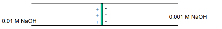
For example, a porous glass frit may separate two solutions of NaOH:

NaOH (0.01 M) // NaOH (0.001 M)

OH^- moves approximately 5X faster than Na⁺ . . .

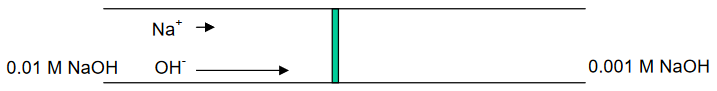
. . . developing of a potential at the interface, or boundary, between the two solutions.

So now for an electrochemical cell containing a salt bridge, the cell potential is actually:

\[E_\ce{cell} = E_\ce{cathode} - E_\ce{anode} + E_\ce{junction} \tag{4}\]

Typical values for a liquid junction potential range from a few mV up to ~40 mV, depending on the identities and concentrations of the electrolyte solutions.

For a simple cell such as the one mentioned on the previous page, the junction potential can be calculated from the ion mobilities. However, most practical electrochemical cells are more complicated. To correct for or minimize errors due to a junction potential you can use the standard addition quantitation method. Here a potential measurement is made on a solution containing just the analyte ion. Next this solution is “spiked” with a known volume of standard ion solution and a second potential measurement is made. This procedure can be continued for multiple spikes (multiple standard addition method). You can assume that the addition of the standard does not alter the junction potential. You can read further about this quantitation method in the Chloride Experiment in the Experimental section of this module.