Metals Analysis by Atomic Spectroscopy

Learning Outcomes

At the end of this assignment students will be able to:

• Understand and apply the underlying theory involved in major areas of atomic spectroscopy.
• Utilize their knowledge of atomic spectroscopy to choose between methods for specific analyses.
• Make use of spreadsheets and graphical analysis to solve problems involving standard addition in elemental analysis.

Purpose

This section will provide an introduction to atomic spectroscopy. The basic concepts of flame atomic absorption spectroscopy (FLAA), graphite furnace atomic absorption spectroscopy (GFAA), and inductively coupled plasma optical emission spectroscopy (ICP-OES) will be presented. Next, the application of each of these techniques to the determination of chromium, copper, lead, and zinc in Lake Nakuru sediment and suspended solid samples will be evaluated and compared to a previous study.

Introduction

Atomic spectroscopy comprises an important set of analytical techniques. The results of atomic spectroscopy experiments are quantitative measurements of elemental concentrations. Because the determination of levels of various metals is important in many clinical assays, products of the food and beverage industry, evaluation of environmental quality and impacts, and in a wide range of manufacturing concerns (from pharmaceuticals to steel), this method is widely applied. Atomic spectroscopy instruments can be divided into three basic types, depending on whether the phenomenon measured is based on light absorption, emission or fluorescence. Although atomic fluorescence can provide lower detection limits for some metal ions, these instruments are less commonly available therefore, our discussion in this unit will focus on analysis using atomic absorption and emission techniques.

Starting small. We all learned in our first course in chemistry that the most basic forms of matter are the elements, and that the smallest unit of an element is the atom. Elements display properties unique to themselves, including the number of electrons located in what are referred to as atomic orbitals. These atomic orbitals are designated by type and energy as 1s, 2s, 2p, 3s, 3p, 4s, 3d, etc.

Q1. Give the electron configuration for sodium (Na, element number 11). In what atomic orbital does the electron with the most energy reside?

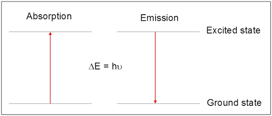
The electron configuration you just wrote for the sodium atom describes the element in its lowest energy or ground state. Each of the atomic orbitals for an element is separated from the next by a discrete or quantized amount of energy, with the energies separating successively higher energy orbitals being different but also discrete. Only when the energy of radiation interacting with an atom exactly matches the gap between two energy levels of the atom will an absorption (or emission) event occur. Not surprisingly, these energy differences are unique to an individual element, and thus can be used to identify that element.

Atomic spectroscopy is based on the quantized changes in atomic energy following the absorption (or emission) of light. In absorption, the energy of the atom increases as an electron is promoted from an orbital of lower energy (the ground state) to one of higher energy (the excited state). In this process, light of the appropriate frequency, \(\nu\), (or wavelength, \(\lambda\)) is absorbed according to Equation \ref{1}, where ΔE represents the difference in energy (in Joules) between the excited and ground states, h is Planck's constant (h = 6.626 × 10^-34 J s), and c is the speed of light in a vacuum (c = 2.998 × 10⁸ m/s).

\[\mathrm{\Delta E = h\nu = \dfrac{hc}{\lambda}} \label{1}\]

Q2. For the sodium atom, if an appropriate amount of energy were absorbed, to what atomic orbital would an electron be promoted if the lowest energy excited state were the result of the absorption?

Q3. Given that the energy difference between the ground state and the first excited electronic state (ΔE) for the sodium atom is 3.373 × 10^-19 J, calculate the frequency, \(\nu\), corresponding to a photon possessing this energy. Next, calculate the wavelength (in nm) for this photon.

Atomic emission is, in essence, the reverse of the absorption process. Atoms in the excited state will emit (or give off) light when the electron relaxes back to the lower energy ground state. Again, because this energy is quantized, the light emitted is of a specific frequency, indicated by Eq 1.

A graphical depiction of this process is provided in Figure 1.

Figure 1. Illustration of the absorption or emission of light by an electron undergoing transitions between the ground and excited electronic states.

Astronomers were among the first to recognize the potential of atomic spectroscopy measurements for elemental analysis. We normally see the light from stars (like our sun) as white light. This light appears white because it is comprised of a continuum of all wavelengths. However, astronomers realized if they carefully analyzed the wavelengths of light emitted by a star, there were missing frequencies, or lines, at very specific wavelengths that corresponded to absorption of light by elements in the atmosphere. (For a more detailed discussion, and example calculations see Harvey, Analytical Chemistry 2.0, Chapter 10, Section 10.1.1.)¹

It is important to remember that in the analysis of Lake Nakuru samples, our measurements will not be made for single atoms, as illustrated in Figure 1, but rather will result from the net absorption or emission from the large numbers of a particular atom in our sample, called a population. Within this population, the fraction of the atoms that will be in the ground or the excited state depends on the sample temperature as defined by the Boltzmann equation, Equation \ref{2}, where N_ground is the population of atoms in the ground state, N_excited is the population of atoms in the excited state, ΔE is the difference in energy between the two states (E_excited - E_ground), T is the temperature in Kelvin and k is the Boltzmann constant (1.381 × 10^-23 J/K).

\[\mathrm{\dfrac{N_{excited}}{N_{ground}} = e ^{- \Delta E/kT}} \label{2}\]

Q4. A common unit for metal analysis is parts-per-million, or ppm. For solids ppm is expressed as mg/kg while for aqueous solutions mg/L is used. The current maximum contaminant level (MCL) set by the EPA for lead in drinking water is 0.015 mg/L.² At this concentration, how many atoms of lead are present in 1 L?

Q5. A common wavelength used for measuring lead emission is 220.353 nm.

1. Calculate ΔE (Joules) for this transition.
2. Calculate the ratio of atoms in the excited state to atoms in the ground state for this value of ΔE at room temperature (298K).
3. Repeat the calculation at 6000K, a routine operating temperature for an ICP torch.
4. Can you hypothesize as to why atomic emission measurements are generally made at high temperatures?

A Short Aside: Atomic vs. Molecular Spectroscopy

In order to better understand atomic spectroscopy, you will want to know how it differs from molecular spectroscopy, a technique you may be more familiar with. Start by considering the differences between atoms and molecules.

Q6. What are molecules?

Simply put, molecules are the combination of atoms that result when bonds are formed between the atoms. Long ago, you learned that when atoms approach each other and their valence electron densities begin to overlap (bonding), atomic orbitals can be combined to form molecular orbitals (remember, for example, s + p = sp). Without going into detail here, since our focus is on atomic spectroscopy, the formation of bonds introduces many, many more possible electron energy levels that can be addressed by the absorption or emission of radiation. In addition to the electronic ground and excited states possible for atoms, molecules possess both vibrational and rotational levels within each of the electronic states, with the energy separations between these new levels much lower than those between the electronic ones.

Since the atomic orbitals are discrete and few in number, atomic spectra consist of very narrow absorption bands at single wavelengths corresponding to the various ΔE values between the orbitals. Molecular spectra are much more complicated than atomic spectra as a consequence of the increased number of accessible energy levels for molecules. Broad absorption bands composed of many, many individual transitions centered on the most favorable absorption wavelength characterize these spectra. This difference is illustrated in Figure 2, below.

Figure 2. Top) Atomic orbitals and corresponding atomic transitions for the sodium atom.¹

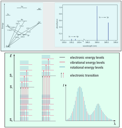
Bottom) Illustration of (left) energy levels for a molecule, with S_o representing a singlet ground state for the molecule and S₁, S₂ representing singlet excited state energy levels, and (right) shape of a typical molecular absorption spectrum.³

The narrow absorption lines for atomic spectroscopy provide its major advantage over molecular spectroscopy. There is rarely any overlap between the spectra of different elements in a complex sample, and with the appropriate detection system, as many as 80 elements can be determined in the same sample rapidly in sequence, or in many cases, simultaneously.

Techniques for Atomic Spectroscopy

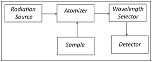
A common goal for all techniques in atomic spectroscopy (AS) is the isolation and quantification of unbound, gas phase atoms from the sample matrix regardless of how the atoms were combined in the sample. The block diagram in Figure 3 lists the general components needed to perform atomic spectroscopy.

Figure 3. Block diagram of an instrument for atomic spectroscopy.

Typically, a liquid sample is introduced into the atomizer through a nebulizer (FLAA, ICP) which breaks the liquid into small particles that can easily be evaporated in either a flame or a plasma. In GFAA, microliter volumes of liquid sample are introduced directly into a small graphite tube (approximately 0.7 x 3 cm) using a micropipettor or autosampler. Atomization is accomplished in the high temperature of the flame (2300 – 3400 K) or the plasma (6000 – 8000 K), or by electrothermal heating in the graphite tube (1500 – 3000 K).

Q7. Consider the relative temperatures of the three atomization sources described in the previous section. Are there cases in which higher temperatures might cause something other than atomization? What group(s) of elements would you expect to be most susceptible?

1. Flame Atomic Absorption Spectroscopy (FLAA) In FLAA, atoms of interest are isolated, or atomized, in a flame. A variety of fuels and oxidants can be used to produce the flame, with the choice dependent upon the desired temperature, which in turn is dependent upon the atom under consideration. Routine analysis can be accomplished with an acetylene/air flame which has a temperature of approximately 2500 K. A “slot” burner is common, which allows for an optical path length across the flame of up to 10 cm. An acetylene/air flame is shown in Figure 4.

The burner assembly for FLAA consists of fuel and oxidant lines (at bottom left in Figure 4) which introduce the gases into the nebulizer where they are mixed and fed into the slot burner head, where they are ignited. The updraft caused by the flame pulls the liquid sample through a small “sipper” (at center of black nebulizer) into the nebulizer where large droplets are eliminated, and the smaller liquid droplets swept into the flame. The flame serves to strip away the solvent and causes atomization of the sample. On either side of the flame are quartz windows that allow the excitation source (at left) to pass through the flame and into the radiation detector (at right). The large clear tube at bottom center is the waste collection line for excess sample.

Figure 4. Burner assembly for FLAA.

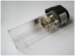
The most common radiation source for FLAA is the hollow cathode lamp (HCL) which incorporates two electrodes inside an evacuated tube containing an inert gas at 1 – 5 torr. The cathode is made from the element of interest, or coated with that element and is maintained at a potential of about 500 V negative of the anode. This applied potential is sufficient to ionize the fill gas molecules (Ar → Ar⁺ + e^-, for example), with the ions being accelerated towards the negatively charged cathode. The inert gas cations strike the cathode with enough force to “sputter” excited state atoms of the element of interest into the gas phase. These excited state atoms emit radiation of characteristic wavelengths that are used to excite gas phase atoms in the flame, with the amount of radiation absorbed by the sample being proportional to the concentration of the atom in the sample. In FLAA, a different HCL is most often required for each element you wish to analyze. A typical lamp is shown in Figure 5.

Figure 5. A typical hollow cathode lamp. The cathode is at the center, the cylindrical shape of which helps direct the emitted radiation towards the end of the tube, most often a quartz window. Dual anodes are located on either side of the cathode.

Single-element lamps limit FLAA to sequential analysis if more than one element is to be determined in a sample. The advantage of narrow, specific absorption bands, however, allows for simple detection systems to be employed. Typically, a minimal monochromator and photomultiplier tube detector suffice for routine analyses.

Q8. Speculate as to possible sources of background interference when using FLAA. How might they be eliminated or reduced?

In FLAA, the primary interference is from the continuum emission from the flame itself. It is possible to distinguish the signal originating in the flame from that of the atomic absorption by electronically pulsing the source lamp (HCL) on and off, and subtracting the signal from the flame from that produced by the combination of the flame + the lamp. A mechanical chopper can also be used for this purpose. Alternatively, background absorption in the flame can be minimized by use of a continuum source (usually a D₂ lamp) alternated with the HCL.⁴ The element being determined effectively absorbs light from the primary source only, while background absorption occurs equally with both beams. The difference between the two signals gives the true atomic absorption signal.

You were asked in Q7 to consider what processes might occur in addition to atomization as the temperature of the atomizer increased. One possibility is that enough energy is transferred to the atoms that they are promoted to an excited energy state. This occurs in the flame primarily for the alkali and alkaline earth elements, whose excitation energies are the lowest. Consequently, these elements can be determined using flame atomic emission spectroscopy (FLAE), where the radiation emitted from the excited state atoms is measured. In a previous course you may have performed flame tests in which you visually observed the color of light emitted when solutions containing metals such as lithium, sodium, potassium or calcium were introduced into a flame using an inert wire loop. You will see in a later section that excitation and ionization occur at the very high temperatures of the ICP, making that atomizer most effective for atomic emission spectroscopy, and for ion detection by mass spectrometry. The development of ICP-based spectroscopy has allowed it to mostly replace FLAE for routine analysis, except in cases where cost is a factor or the increased sensitivity of the ICP is unnecessary. Figure 6 shows the red emission of atomic lithium in an acetylene/air flame.

Figure 6. Lithium emission in an acetylene/air flame.

2. Graphite Furnace Atomic Absorption Spectroscopy (GFAA) The graphite furnace is generally a cylindrical graphite tube placed in the optical path of the spectrophotometer, with rapid atomization accomplished by the application of high electrical potential at two contact points. Two types of tubes are in common use: a) the transversely heated graphite tube in which the electrodes are applied perpendicular to the light path, allowing for even heating along the entire length of the tube, and b) the longitudinally heated tube where electrode contacts are at the ends of the tube, frequently resulting in uneven heating. Both types of tube are shown in Figure 7.

Figure 7. Left) Transversely heated graphite tube. Right) Longitudinally heated graphite tube.

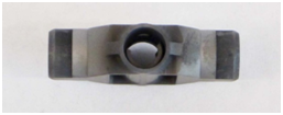
The graphite tube is commonly fitted with what is called a L’vov (after its inventor) platform, a curved surface attached at a single point to the outside walls of the tube which allows for the sample to be heated radiatively as the temperature is increased. This results in more even heating of the sample and better reproducibility of response. The platform can be seen in Figure 8.

Figure 8. The L’Vov Platform

Aliquots of liquid sample (5 – 50 μL) are introduced through a small hole located in the center of the tube. The technique is also amenable under certain conditions to solid samples. The GFAA assembly is mounted within an enclosed, water-cooled housing so that temperature can be quickly lowered between runs. Inert gas, typically argon, is used to protect the tube from oxidation at high temperatures, and to purge oxygen from the tube to prevent the formation of metal oxides during the atomization step. One type of furnace arrangement is shown in Figure 9.

Figure 9. Graphite furnace assembly. The transversely heated tube is located at the center of the figure (black), with electrode contacts above and below. The grey cylindrical structure is a water cooled jacket, also enclosing an electromagnet used in Zeeman noise correction. The tubes at top right and left supply cooling water, while the lines at bottom supply argon both internal and external to the tube.

The furnace typically allows 2 – 3 orders of magnitude lower limits of detection than the flame, and requires significantly less sample.

Q9. How does the design of the graphite furnace allow for such improved sensitivity for metals over flame AA?

Normally, a GFAA measurement is made in five steps. The first of these is the drying step, in which the temperature of the furnace is raised slowly to a temperature slightly above the boiling point of the solvent, and held there for 30 – 60 seconds. Some methods specify that this step be repeated at a temperature slightly higher than the first drying temperature to assure complete solvent removal and to prevent “bumping” at higher temperatures. The second step is referred to as the charring step, in which the organic compounds and other low boiling substances in the sample are thermally decomposed. The charring, or pyrolysis temperature is typically between 600 and 1000 ^oC. Argon is allowed to flow through the tube during these first two steps to remove smoke and other vapors produced in drying and pyrolysis. The third step, atomization, is dependent somewhat upon the element of interest, but is routinely between 1500 and 2000 ^oC. The argon flow is stopped during the 5 – 10 second measurement window, trapping the atomized sample in the small volume of the graphite tube where its absorbance is integrated over time. After the sample has been atomized, the temperature is raised quickly to a value several hundred degrees higher than the atomization temperature and held there for 10 – 20 seconds with a high rate of argon flow. This clean out step assures that any sample residue remaining in the tube is removed. The last step is the cool down step in which the furnace is allowed to return to ambient temperature (with water cooling) before the next sample is introduced.

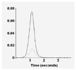
The GFAA signal observed for Pb at a concentration of 5 μg/L is shown in Figure 10. In contrast to FLAA, where the observed absorbance signal for a sample is constant as long as the sample is being aspirated, the observed signal in GFAA is transient as a result of atomization of the entire amount of analyte during the measurement step. The signal increases during atomization, and then decreases as the vaporized atoms diffuse out of the furnace. Generally, the integrated peak area (AU x s) is used in quantification of the element of interest.

Figure 10. GFAA signal observed for 40 μL sample containing 5 μg/L of Pb (200 pg). The lower trace is the background signal observed for 0.2% v/v HNO₃.⁵

Most GFAA methods include the addition of a matrix modifier to the sample volume introduced into the furnace. Matrix modifiers reduce the loss of analyte during charring by enhancing the volatility of the matrix so that it is removed at a lower temperature or by making the analyte less volatile so that a higher atomization temperature can be employed. Commonly used matrix modifiers include palladium metal and Mg(NO_3­)₂. Dilute solutions of these modifiers, on the order of 0.1% m/v, are added in small amounts to the sample being analyzed. Added masses of modifiers range from 3 – 50 μg in the analyzed sample volume, depending upon the analyte.

Generally, the same detection system can be used for GFAA as for FLAA. Similarly, most GFAA systems will employ the same D₂ continuum correction. In addition, many GFAA systems include what is known as a Zeeman correction system that allows background correction at higher absorbance values than D₂ correction, and for matrices that are more spectrally complex. Zeeman correction is also applicable at all wavelengths.⁶ Figure 11 shows the instrumental arrangement for one type of Zeeman correction.

Figure 11. Zeeman correction for GFAA. The two poles of an electromagnet are placed on either side of the furnace, with the magnetic field pulsed on and off during the atomization step.⁷

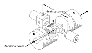
The basis for Zeeman correction is the observation that the absorption (or emission) bands observed for atoms can be split into multiple lines in the presence of an applied magnetic field. In the simplest example, a single absorption band can be split into two components observed at slightly lower and slightly higher wavelengths than the original. By pulsing the magnetic field during the atomization step, the signal observed at the original wavelength when the magnet is on (background only) can be subtracted from the signal observed when the magnet is off (background + analyte) to give the corrected signal.

3. Inductively Coupled Plasma – Optical Emission Spectroscopy (ICP-OES) The atomization source for this technique, known as an inductively coupled plasma, operates at significantly higher temperatures than do the flame and the furnace. As a result, many of the atoms are excited into higher energy states, making this technique more amenable to the measurement of emission rather than absorption. Since the plasma can serve as both the atomizer and the excitation source, a separate source like the HCL is unnecessary in this technique.

As we will see, the sensitivity and dynamic range of this technique are far better than either of the two we have studied previously. Except for its much higher initial cost and an increased cost of routine operation, this method satisfies nearly every critical figure of merit for atomic spectroscopy.

Figure 12. Schematic diagram of an inductively coupled plasma torch.¹

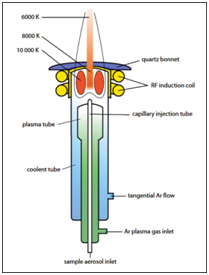
Plasma is a distinct phase of matter, composed of highly ionized gas containing high concentrations of ions and free electrons. The plasma for ICP is initiated by ionizing a flowing stream of argon by the injection of free electrons with a Tesla coil. The high energy of the plasma is maintained by inducing the charged particles to rotate within a fluctuating magnetic field generated in an RF (radio frequency) coil. Resistance to this motion by unionized argon generates considerable resistive heating resulting in temperatures of 6000 - 10,000 K. A schematic of an ICP torch is shown in Figure 12.

It is composed of concentric tubes, generally quartz, allowing three distinct paths of argon flow. The inner gas flow, through the capillary injection tube, carries the sample aerosol from the nebulizer into the plasma. An intermediate gas flow, through the argon plasma gas inlet, serves to keep the plasma localized above the injection tube and away from the intermediate flow tube. This flow also reduces the buildup of carbon at the injector tip when organic samples are introduced.⁸ The outer flow, labeled Ar tangential flow in Figure 12, serves to keep the quartz walls of the torch cool. Because of the small spacing between the intermediate and outer flow tubes, argon follows a tangential path through the tube at high velocity.

As was mentioned before, the energy of the plasma is sufficient to populate many excited states of resident atoms at the same time, making ICP-OES an ideal method for multielement analysis. For many elements significant numbers of excited state ions also result. This generally allows for multiple spectral lines to be available for each element, with many elements emitting most strongly from excited ionic states. Quantitative information is obtained most commonly from comparison of emission intensity of unknown to calibration plots of emission intensity as a function of concentration. Linear calibration plots for ICP-OES are linear over 4 – 6 orders of magnitude, superior to both FLAA and GFAA.

Figure 13 shows the ICP torch assembly mounted inside an ICP-OES instrument. This arrangement has the torch installed horizontally, with the nebulizer flow entering at the left. Two of the argon flow lines are visible at bottom left, with the copper induction coil wrapped around center of the glass torch.

Figure 13. Instrumental configuration of ICP torch in an ICP-OES.

The instrument illustrated in Figure 13 allows two different optical paths by which emitted radiation can be measured. At right, the cylindrical window allows introduction of radiation to the detector from an axial direction, that is, head-on to the top of the ICP torch. An alternative pathway allows radiation to be measured radially to the torch, with the optical window leading to the detector located at a right angle to the torch, center bottom of figure. This design allows for a wider dynamic analytical range, with the axial arrangement giving better linearity of response at low concentrations of analyte, resulting from the increased path length through the torch from which the emission is being measured. The radial path allows for the best linearity of response at high concentrations of analyte.

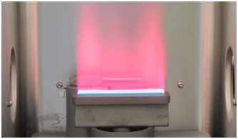
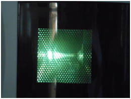
The argon ICP plasma torch displays a very intense continuum emission that appears white in color. A photograph of the torch in operation is found in Figure 14.

Figure 14. ICP plasma torch in operation.

Detection systems in ICP-OES most commonly employ a diffraction grating that allows radiation emitted from the elements in the plasma to be directed onto either multiple PMTs or high sensitivity solid state detectors for simultaneous intensity measurement at multiple wavelengths. Included in the latter type are the photodiode array detector (PDA), the charge injection device (CID), and the charge coupled device (CCD). A complete discussion of detector systems for emission spectroscopy can be found in reference 9.⁹

For ICP-OES, most chemical interferences are eliminated by the high temperature of the plasma. Background emission from the plasma itself can be easily removed by subtraction of the emission intensity at a position away from an emission line of interest from the intensity at the emission line. This is especially straightforward for one of the solid state detection techniques that measure a continuous background across a band of wavelengths. Spectral interferences can most often be minimized or eliminated by selection of a different wavelength band for the observation of emission intensity for an element of interest. Having multiple bands to choose from for each element also lends itself well to improving linearity of response, where a weaker emission band can be chosen for high concentration species in the sample.

Summary

An excellent guide to the strengths and limitations of FLAA, GFAA, and ICP-OES (as well as additional techniques not covered in this module) can be found in Reference 13. A general decision matrix for choice of method reprinted from that source is given below as Table 1.¹³ A comparison of several important instrumental parameters for FLAA, GFAA, and ICP-OES are found in Table 2. Lastly, specific information on the achievable limits of detection (LOD) and limits of linearity (LOL) for the four metals being considered here are included for the three techniques in Table 3.

Table 2. Important Instrumental Parameters for FLAA, GFAA, and ICP-OES¹³

	FLAA	GFAA	ICP-OES
Detection Limit Ranges	0.9 – 100 ppb	0.005 – 2 ppb	0.02 – 100 ppb
Typical System Costs	$15 – 25K	$30 – 50K	$60 – 100K
Analytical Working Range* (orders of magnitude)	4	2.5	10

*concentration range over which quantitative results can be obtained without recalibration

Table 3. Comparison of Detection Limits (LOD) and Limit of Linearity (LOL) for FLAA, GFAA, and ICP-OES (all values are in μg/L, ppb)

	FLAA		GFAA		ICP-OES
Metal	LOD^13	LOL^*	LOD^13	LOL^*	LOD^13	LOL^15
Cr	1.5	10^4	0.014	4.4	0.4	10^5
Cu	3.0	10^4	0.004	1	0.2	10^5
Pb	15	10^5	0.05	16	1	10^5
Zn	1.5	10^4	0.02	6	0.2	10^5

* Limits of linearity for AA and GFAA are estimated from analytical working range estimates in Reference 13.

Data and Analysis

In the following section, you will evaluate the data reported in Nelson, et al.¹⁰ for the analysis by atomic spectroscopy and XRF of Cr, Cu, Pb, and Zn in suspended solids and dried sediments from Lake Nakuru. Next, you will be supplied with simulated data from sediments and suspended solids so that you can compare those levels of the four target metals to those obtained in 1996. As a starting point, let us look again at the results from that previous investigation.

The procedure used by Nelson to prepare samples of Lake Nakuru sediments and suspended solids for analysis by atomic spectroscopy can be summarized as follows:

5 g samples of filtered and dried solids were digested for 1 hour in 50 mL of high purity HNO₃. The digested samples were filtered through 0.45 μm PVDF membranes and the filtrate diluted to a final volume of 50.00 mL in a volumetric flask with purified water.

Final concentrations for each of the four metals found in sediments and suspended solids by Nelson are given in Table 4 on a dry weight basis (μg/g). The results for Lake Nakuru suspended solids were obtained using XRF, a technique you will encounter in a separate section of this module.

Table 4. Metal Concentrations in Lake Nakuru Sediments and Suspended Solids found in Nelson Study¹⁰

	Concentration in dry sediments (µg/g)		Concentration in suspended solids (µg/g)
Trace metal	Average (11 sites)	Range	Average	Standard deviation
Chromium	67	10 – 280	8.3	0.82
Copper	24	5 – 95	19	2.9
Lead	22	4 – 100	11.7	0.9
Zinc	147	44 – 630	74	31

Q10. For the metals in Table 4, use the average final dry concentration to calculate the dissolved concentration (mg/L, ppm) of each metal in a liquid sample prepared from 5.00 g of dried sediment or suspended solids diluted to a final volume of 50 mL for analysis by atomic spectroscopy.

The concentrations you calculated in Q10 for each of the metals in sediment and suspended solids may suggest to you which method you learned about earlier in this module would be most appropriate for each of the metals if further study were performed.

Q11. If no further information were given, which technique would be your first choice in measuring the concentration of the four metals in both of the matrices if you were to perform a follow-up study to that done by Nelson? Explain your choice(s).

Returning to the Nelson paper, if you dig further into the procedure for suspended sediment sample preparation beyond the initial 50 mL dilution you will find the following:

…samples were diluted with distilled-deionized water (10 to 50x) to reduce observed matrix effects, and the method of standard additions was used to account for any remaining matrix effects.

This additional dilution was required in the analysis for each of the metals except for Zn, for which no further dilution was required to reduce observed matrix effects.

Q12. In general, what are matrix effects? What about the chemistry of Lake Nakuru might be the cause of the severe matrix effects observed for measurements of Cr, Cu, and Pb by atomic spectroscopy?

Q13. Which of the three methods you have studied is best able to overcome matrix effects? Why is this so?

Q14. If the original 50 mL digestion solution, for which you calculated metal concentrations previously, were further diluted by a factor of 50x to reduce matrix effects, would this alter your answer(s) from Q11 as to choice of method for Cr, Cu, and Pb?

Simulated Analysis of Present-day Lake Nakuru Metals

As a follow-up to the study conducted by Nelson, et al. on samples collected from Lake Nakuru in 1996, you will now have a chance to evaluate simulated data for Cr, Cu, Pb, and Zn levels in sediments and suspended solids. You may have come to the conclusion in the previous section that the best method available to evaluate multiple metal species in complex matrices is that of ICP-OES. EPA Method 200.7 (Revision 4.4) Determination of Metals and Trace Elements in Water and Wastes by Inductively Coupled Plasma-Atomic Emission Spectrometry¹¹ will be the method of choice for this analysis. It can be obtained free online here.

The method is applicable to 32 metals, including the four of interest, in various matrices. For this study, it has been applied to samples of sediment and filtered suspended solids that were dried to constant weight at 60 ^oC. In our analysis, 1 gram samples of solid were massed exactly and digested in nitric and hydrochloric acids, then taken up into a final volume of 100 mL. The one exception was that for analysis of lead in suspended solids – in that case, a 3 gram sample was required to provide an appropriate instrument response.

Table 1 of Method 200.7 gives the optimal wavelength for each of the metals, along with an estimated method detection limit (LOD) and an upper concentration limit to which calibration plots are typically linear (LOL). Normally, the lowest concentration that is reliably quantitated (LOQ) is taken as 10x the method detection limit.

Q15. Suppose you were to construct calibration plots for each of the four metals of interest in this study between the LOD and LOL values suggested in Method 200.7. Would 1 gram samples of Lake Nakuru sediment with the metal concentrations found in the 1998 report (Table 4 of this module), diluted to a final volume of 100 mL, have analyzed values that fall between the limits on these calibration plots?

Because matrix effects were an issue in the 1998 report, we have chosen to use the method of standard additions in the measurement of metal concentrations by ICP-OES. Background information on standard addition methods can be found in Harvey, Chapter 5.¹²

Sediment samples. Four 1.0000 g samples of dried sediment were accurately massed into separate digestion vessels, and treated according to Method 200.7. Following the extraction, the liquid extracts were quantitatively transferred to separate 100 mL volumetric flasks. Standard additions were then made for each of the four metals so that the four flasks had final added standard concentrations of 0.00, 0.10xLOL, 0.20xLOL, and 0.50xLOL (all in ppm). For example, zinc was added in sufficient quantities to give final added concentrations of 0.00, 0.50, 1.00 and 2.50 ppm following dilution to 100 mL with reagent water. 1000 ppm standards for each metal (ICP grade) can be obtained commercially or prepared according to instructions in Section 7.0 of Method 200.7.¹¹

Suspended solid samples. Analysis of Cr, Cu, and Zn: four 1.0000 g samples of dried suspended solids were treated in the same way as for sediment (previous section). Standard solutions were added at the same levels as before in each of the four volumetric flasks prior to dilution with reagent water. Analysis of Pb: four 3.0000 g samples of dried suspended solids were digested as before, transferred to separate 100 mL volumetric flasks, appropriate amounts of Pb standard added to each flask, and dilution to final volume accomplished with reagent water.

All samples were then analyzed sequentially using the ICP-OES conditions specified in Sections 10.1 and 10.2 of Method 200.7.¹¹ A spreadsheet file will be supplied to you that contains tables of emission intensity, corrected for background, as a function of added standard concentration of each element.

Q16. Use the graphical method for multiple standard additions to constant final volume to determine the concentrations of each of the four metals in Lake Nakuru sediments and suspended solids. This graphical method is discussed in Harvey, Chapter 5.¹² Prepare a table of concentrations similar to Table 4 in this module for the most recent concentrations. How have the concentrations of each changed since 1998?

References

1. Harvey, David Analytical Chemistry 2.0, Spectroscopy, Chapter 10, http://www.asdlib.org/onlineArticles.../Chapter10.pdf, accessed June 26, 2012.
2. Drinking Water Contaminants, U.S. EPA, http://water.epa.gov/drink/contaminants/index.cfm, accessed June 25, 2012.
3. Fundamentals of UV-visible Spectroscopy, Primer, Tony Owens, Agilent Technologies, 2000, p. 6, http://www.chem.agilent.com/Library/primers/Public/59801397_020660.pdf, accessed 6/5/2012.
4. Harris, Daniel C.Quantitative Chemical Analysis, 7^th Edition, W. H. Freeman, New York, 2007, 465-466.
5. AAnalyst 800 Detection Limits – Lead Data. Perkin- Elmer Instruments, Technical Note D6204, 2000.
6. Concepts, Instrumentation and Techniques in Atomic Absorption Spectrophotometry, 2^nd Edition, Richard D. Beaty and Jack D. Kerber, Perkin-Elmer Instruments, 1993.
7. THGA Graphite Furnace Users Guide, Perkin-Elmer Instruments, 2000.
8. Concepts, Instrumentation and Techniques in Inductively Coupled Plasma Optical Emission Spectrometry, 2^nd Edition, Charles B. Boss and Kenneth J. Fredeen, Perkin-Elmer Instruments, 1997.
9. Atomic Emission Spectroscopy, Alexander Scheeline and Thomas M. Spudich, http://www.asdlib.org/learningModules/AtomicEmission/index.html, accessed June 25, 2012.
10. Nelson, Y. M. et al.Environmental Toxicology and Chemistry 1998, 17(11), 2302-2309.
11. Martin, T. D., Brockhoff, C. A., Creed, J. T., EPA Method 200.7 (Rev. 4.4), www.epa.gov/sam/pdfs/EPA-200.7.pdf, accessed September 18, 2012.
12. Harvey, David, Analytical Chemistry 2.0, Standardizing Analytical Methods, Chapter 5, http://www.asdlib.org/onlineArticles...s/Chapter5.pdf, accessed September 18, 2012.
13. Atomic Spectroscopy: A Guide to Selecting the Appropriate Technique and System, http://www.perkinelmer.com/PDFs/Downloads/BRO_WorldLeaderAAICPMSICPMS.pdf, accessed June 5, 2013.
14. Harris, op. cit., p. 87.
15. Increased Laboratory Productivity for ICP-OES Applied to U.S. EPA Method 6010C, http://www.perkinelmer.com/CMSResources/Images/44-74168APP_ICP-OESAppliedtoEPAMethod6010C.pdf, accessed June 8, 2013.

Resources

• Data (Excel, PDF)
• Results (Excel, PDF)