Linear Regression

Introduction

In lab you frequently gather data to see how a factor affects a particular response. For example, you might prepare a series of solutions containing different concentrations of Cu²⁺ (the factor) and measure the absorbance (the response) for each solution at a wavelength of 645 nm. A scatterplot of the data

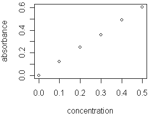
shows what appears to be a linear relationship between absorbance and [Cu²⁺]. Fitting a straight-line to this data, a process called linear regression, provides a mathematical model of this relationship

\[\mathrm{absorbance = 1.207\times[Cu^{2+}] + 0.002}\nonumber \]

that can be used to find the [Cu²⁺] in any solution by measuring that solution's absorbance. For example, if a solution's absorbance is 0.555, the concentration of Cu²⁺ is

\[\mathrm{0.555 = 1.207\times[Cu^{2+}] + 0.002}\nonumber \]

\[\mathrm{0.555 - 0.002 = 0.553 = 1.207\times[Cu^{2+}]}\nonumber \]

\[\mathrm{\dfrac{0.553}{1.207} = [Cu^{2+}] = 0.458\: M}\nonumber \]

A scatterplot showing the data and the linear regression model

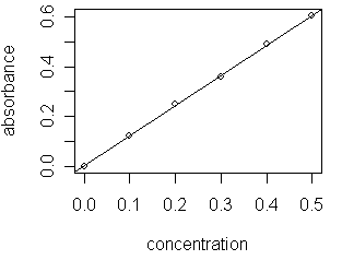
suggests that the model provides an appropriate fit to the data. Unfortunately, it is not always the case that a straight-line provides the best fit to a data set. The purpose of this module is to emphasize the importance of evaluating critically the results of a linear regression analysis.

After you complete this module you should:

• appreciate how a linear regression analysis works
• understand that it is important to examine visually your data and your linear regression model

Before tackling some problems, read an explanation of how linear regression works.

Data

Here is the data used in this example:

[Cu^2^+] (M)	Absorbance
0.000	0.000
0.100	0.124
0.200	0.248
0.300	0.359
0.400	0.488
0.500	0.604

• How It Works

• Problem 1

• Problem 2

• Problem 3

• Summary

• Further Study