
Statistics (Witter)
- Page ID
- 279687

Introduction to Statistics I
Learning Goals:
- To understand how a sample relates to a population;
- To understand how a population can be represented by the normal distribution according to the Central Limit Theorem
- To understand how a confidence interval can be used to indicate where the true mean is found for a sample
Samples and Populations
When we make chemical measurements, we often have a finite amount of time or money or both in terms of collecting and measuring samples. In most analyses, we are limited to measuring a portion (sample) of all the material present (population). The question becomes: How well does the sample represent the larger population? If we look at the distribution of the measurements we made, we can gain insight into the population.
Probability Distributions in Chemistry
The two most important types of probability distributions in chemistry are binomial distributions, which have fixed values, and normal distributions, which have a range of possible values. We will focus on normal distributions from here forward. When we make measurements of a sample from a population, we are unlikely to make a large enough set of measurements to fully represent the population. But, if we make enough sample measurements, and only random errors are present, the resulting mean and variance should approximate the normal distribution of the population. That is, for a series of sample measurements in which only random errors are present, the data will approximate a normal distribution based on probability theory – called the Central Limit Theorem. The Central Limit Theorem states that when a system is subject only to indeterminate error, the results of multiple measurements approximate a normal distribution where 68% of the samples will lie within ± 1 standard deviation of the mean; 95% of samples will lie within ± 2 standard deviations of the mean; and 99% of the samples will lie within ± 3 standard deviations of the mean. As such, samples can approximate attributes of the larger population, such as the mean and variance.
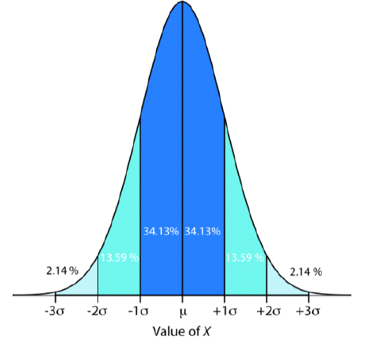
Figure 1. Normal distribution curve from Harvey Analytical Chemistry 2.1
Confidence Intervals (μ)
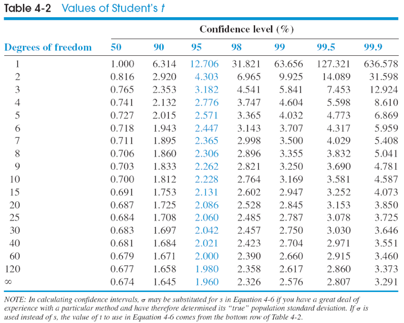
Confidence intervals are ranges where we expect the true mean to lie for a population, based on the mean and standard deviation of a series of sample measurements. Confidence intervals can be determined for different levels of certainty (50%, 90%, 95%, 99%). To calculate a confidence interval, we must know the mean or average value (\(\bar{X}\)) for a set of measurements, the number of measurements (n), a Students’ T value table, and the standard deviation of the set of measurements (s). To calculate a confidence interval, we use the formula:
\[\mu = \bar{X} \pm \dfrac{ts}{\sqrt{n}}\nonumber\]
Where \(\bar{X}\) is the average value of a set of measurements, n is the number of measurements, t is the Students’ t value for n-1 degrees of freedom, and s is the sample standard deviation.
Problems
(From Harvey Analytical Chemistry 2.1; https://community.asdlib.org/activel...line-textbook/)
- The carbohydrate content of a glycoprotein (a protein with sugars attached to it) is found to be 12.6, 11.9, 13.0, 12.7, and 12.5 wt% (g carbohydrate/100 g glycoprotein) in replicate analytes. Find the 50% and the 90% confidence intervals for the carbohydrate content.
- What is the relationship between the standard deviation and the precision of a procedure? What is the relationship between the standard deviation and the accuracy?
- What is the meaning of a confidence interval?
- The percentage of an additive in gasoline was measured six times with the following results: 0.13, 0.12, 0.16, 0.17, 0.20, 0.11 wt%. Find the 90% and the 99% confidence intervals for the percentage of the additive.
Note
Another way the confidence interval equation is used is to compare your experimental result to an accepted (or true) value. For example, assume we measure a quantity several times, and obtain an average value and standard deviation. We need to compare our answer with an accepted answer. Does our measured value agree with the accepted value “within experimental error?” We can use the confidence interval equation to find out.
- You purchase a standard from the National Institute of Standards (NIST) that is certified to contain 3.19% sulfur. You are testing a new analytical method to see whether it can reproduce the known value. The measured values you obtain are 3.29, 3.22, 3.30, and 3.23 wt % sulfur. Does your new method agree with the accepted answer at the 95% confidence interval? (The 95% CI is the default value that most chemists use).
- A new procedure for the rapid determination of sulfur in kerosene was tested on a sample known from its method of preparation to contain 0.123% sulfur. The results for % sulfur were 0.112, 0.118, 0.115, and 0.119. Do the data indicate that there is a bias in the method at the 95% CI?
- Which of the statements below are TRUE regarding the mean and standard deviation?
- As the number of measurements increases, \(\bar{x}\) approaches μ if there is no random error.
- The square of the standard deviation is the average deviation.
- The mean is the center of the Gaussian distribution.
- The standard deviation measures the width of the Gaussian distribution.
- Calculate the mean and standard deviation for the results below for the concentration of lead in a soil sample.
23.2 ppm, 20.1 ppm, 24.7 ppm, 19.9 ppm, 21.8 ppm
- 21.9 ± 3.4 (n = 5) ppm
- 21.9 ± 2.0 (n =5) ppm
- 27.4 ± 2.0 (n = 5) ppm
- 22.0 ± 1.8 (n = 5) ppm
- 27.4 ± 4.2 (n = 5) ppm
- For the statements below, which is(are) TRUE for confidence intervals?
- As the percentage confidence increases, the confidence interval range decreases.
- Confidence intervals are calculated using the calculated mean and standard deviation of a set of n measurements; and the results of the F test.
- The 95% confidence interval will include the true population mean for 95% of the sets of n measurements.
- I only
- II only
- I and III
- I and II
- III only
- The density of a solution is measured six times with the results of 1.098, 1.100, 1.089, 1.095, 1.097 and 1.101 g/mL. Calculate the 95% confidence interval for the density.
- 1.0967 ± 0.0043 g/mL
- 1.0967 ± 0.0038 g/mL
- 1.0967 ± 0.0041 g/mL
- 1.0967 ± 0.0045 g/mL
- 1.0967 ± 0.0039 g/mL
Introduction to Statistics II
Learning Goals:
- To compare two sample means (paired data)
- To compare two sample means (unpaired data)
- To compare sample variances using the F-test
- To use Dixon’s test for outliers to determine when data can be discarded
Students’ T-test
There are many cases in chemistry where two sets of data need to be compared. The question we are typically asking is whether the means of two sets of data are the same or different, within statistical limits. When we perform a Students’ t-test, we are testing the null hypothesis (Ho), which we either accept or reject. The null hypothesis states that indeterminate (random) errors alone are sufficient to explain the differences between means. The alternative hypothesis (HA) says that the differences in our results are too large to be explained by random error alone. In comparing two means, we first need to decide what type of data we are dealing with, paired or unpaired data. Although at first glance this seems easy, it requires some thought as it will affect the choice of t-test one uses to test the null hypothesis.
Paired versus unpaired data
With paired data, the SAME samples are measured once using each technique. With unpaired data, the sample is SPLIT and part of the sample is measured multiple times. One simple test is to look at the number of samples being analyzed to obtain each mean. If the number of samples is different, then the data is unpaired. But the converse is not true; if two sets of data have the same number of samples, the data may be paired or unpaired. You have to read the question carefully and figure out how the experiment was done in order to know which t-test to use.
Using the Unpaired t-test
Once you decide that the unpaired t-test is the test we need to use, you need to make one more decision to determine which form of the unpaired t-test is necessary. There are two equations depending on whether the variances are the same or different. To determine whether the variances are the same or different, you must perform an F-test.
\[F_{exp} = \dfrac{s_A^2}{s_B^2}\nonumber\]
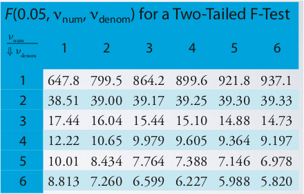
The outcome will be:
- Fexp < Ftable therefore, variances are the same, or
- Fexp > Ftable therefore, variances are different.
Unpaired t-test with pooled variances (i.e. variances are the same)
\[t_{exp} = \frac {|\bar{X}_A - \bar{X}_B|} {s_{pool}} \times \sqrt{\frac {n_A n_B} {n_A + n_B}}\nonumber\]
\[s_{pool} = \sqrt{\frac {(n_A - 1) s_A^2 + (n_B - 1)s_B^2} {n_A + n_B - 2}}\nonumber\]
Unpaired t-test without pooled variances (i.e. variances are different)
\[t_{exp} = \frac {|\bar{X}_A - \bar{X}_B|} {\sqrt{\dfrac {s_A^2} {n_A} + \dfrac {s_B^2} {n_B}}}\nonumber\]
\[\nu = \dfrac {\left[ \dfrac {s_A^2} {n_A} + \dfrac {s_B^2} {n_B} \right]^2} {\dfrac {\left( \dfrac {s_A^2} {n_A} \right)^2} {n_A + 1} + \dfrac {\left( \dfrac {s_B^2} {n_B} \right)^2} {n_B + 1}} - 2 \nonumber\]
V can be rounded to the nearest whole number to determine the d.o.f.
Using the Paired t-test
If the data are paired, the form of the t-test to use is:
\[t_{exp} = \frac {|\bar{d}| \sqrt{n}} {s_d} \nonumber\]
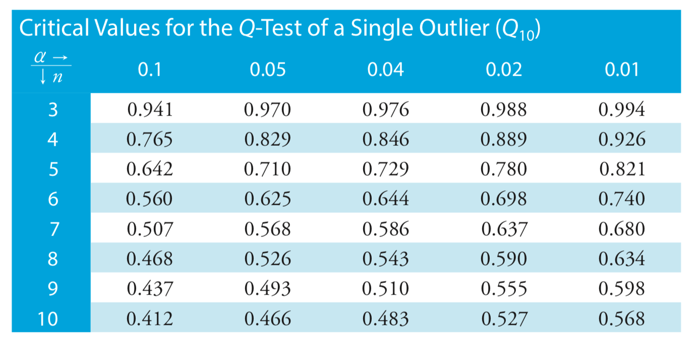
Dixon’s test for outliers
If you are trying to determine if you can throw out a data point you suspect is an outlier, you can use Dixon’s test, where:
\[Q_\text{exp} = Q_{10} = \dfrac {|\text{outlier's value} - \text{nearest value}|} {\text{largest value} - \text{smallest value}} \nonumber\]
Problems
(From Harvey Analytical Chemistry 2.1)
-
Horvat and co-workers used atomic absorption spectroscopy to determine the concentration of Hg in coal fly ash. Of particular interest to the authors was developing an appropriate procedure for digesting samples and releasing the Hg for analysis. As part of their study they tested several reagents for digesting samples. Their results using HNO3 and using a 1 + 3 mixture of HNO3 and HCl are shown here. All concentrations are given as ppb Hg sample.
HNO3 1 + 3 HNO3 – HCl 161 159 165 145 160 140 167 147 166 143 156 Determine whether there is a significant difference between these methods at \(\alpha = 0.05\).
-
Lord Rayleigh, John William Strutt (1842-1919), was one of the most well known scientists of the late nineteenth and early twentieth centuries, publishing over 440 papers and receiving the Nobel Prize in 1904 for the discovery of argon. An important turning point in Rayleigh’s discovery of Ar was his experimental measurements of the density of N2. Rayleigh approached this experiment in two ways: first by taking atmospheric air and removing O2 and H2; and second, by chemically producing N2 by decomposing nitrogen containing compounds (NO, N2O, and NH4NO3) and again removing O2 and H2. The following table shows his results for the density of N2, as published in Proc. Roy. Soc. 1894, LV, 340 (publication 210); all values are the grams of gas at an equivalent volume, pressure, and temperature.
Atmospheric Origin Chemical Origin 2.31017 2.30143 2.30986 2.29890 2.31010 2.29816 2.31001 2.30182 2.31024 2.29869 2.31010 2.29940 2.31028 2.29849 2.29889 Explain why this data led Rayleigh to look for and to discover Ar.
-
One way to check the accuracy of a spectrophotometer is to measure absorbances for a series of standard dichromate solutions obtained from the National Institute of Standards and Technology. Absorbances are measured at 257 nm and compared to the accepted values. The results obtained when testing a newly purchased spectrophotometer are shown here. Determine if the tested spectrophotometer is accurate at \(\alpha = 0.05\).
Standard Measured Absorbance Expected Absorbance 1 0.2872 0.2871 2 0.5773 0.5760 3 0.8674 0.8677 4 1.1623 1.1608 5 1.4559 1.4565 -
Gács and Ferraroli reported a method for monitoring the concentration of SO2 in air. They compared their method to the standard method by analyzing urban air samples collected from a single location. Samples were collected by drawing air through a collection solution for 6 min. Shown here is a summary of their results with SO2 concentrations reported in μL/m3.
Standard Method New Method 21.62 21.54 22.20 20.51 24.27 22.31 23.54 21.30 24.25 24.62 23.09 25.72 21.02 21.54 Using an appropriate statistical test, determine whether there is any significant difference between the standard method and the new method at \(\alpha = 0.05\).
Contributors and Attributions
- Amy Witter, Dickinson College (witter@dickinson.edu)
- Sourced from the Analytical Sciences Digital Library