Statistics (Mullaugh)

Example 1: Average and standard deviation

The following data were recorded for an analysis of the calcium content in a sample of milk. Find the mean, standard deviation and relative standard deviation. Use both the “long way” of finding standard deviation and the function on your calculator to make sure you are using your calculator correctly.

[Ca^2+] / μM
30.5
31.7
31.2
30.8
29.9

 

 

Example 2: Comparing two standard deviations (F-test)

A child is undergoing treatment for lead poisoning. The table below summarizes the results of an analysis of the child’s blood lead level (BLL, in µg/dL) initially and after a month of treatment.

Day	BLL (µg/dL)		n
	mean	st. dev.
0	32.7	0.9	4
30	27.5	0.8	5

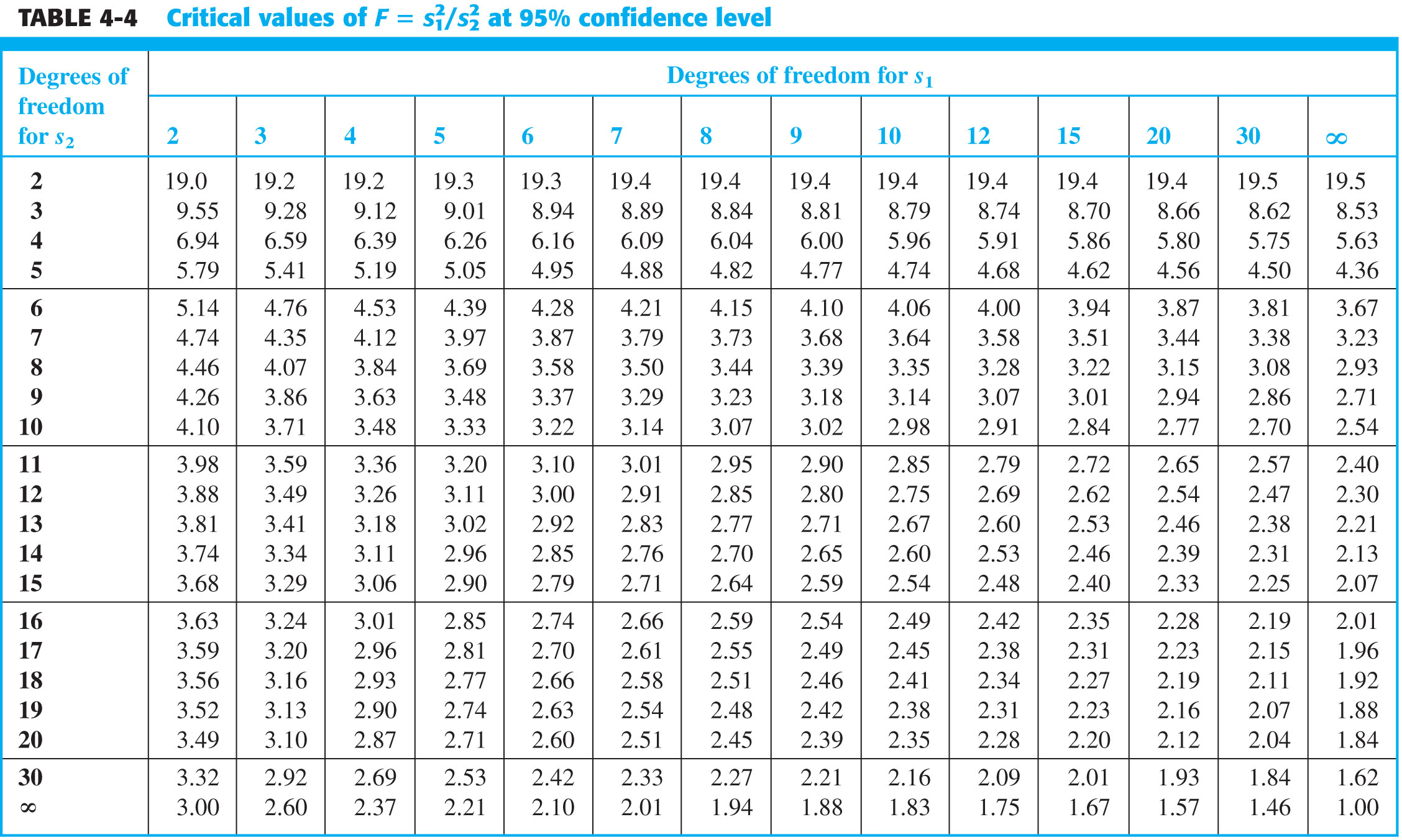
We would like to determine if the treatment is working, but before we compare the average results, we must first determine if the standard deviations are significantly different. Use the F-test to answer this question and indicate the critical value of F used from the table for comparison.

 

 

 

 

 

Example 3: Confidence Intervals

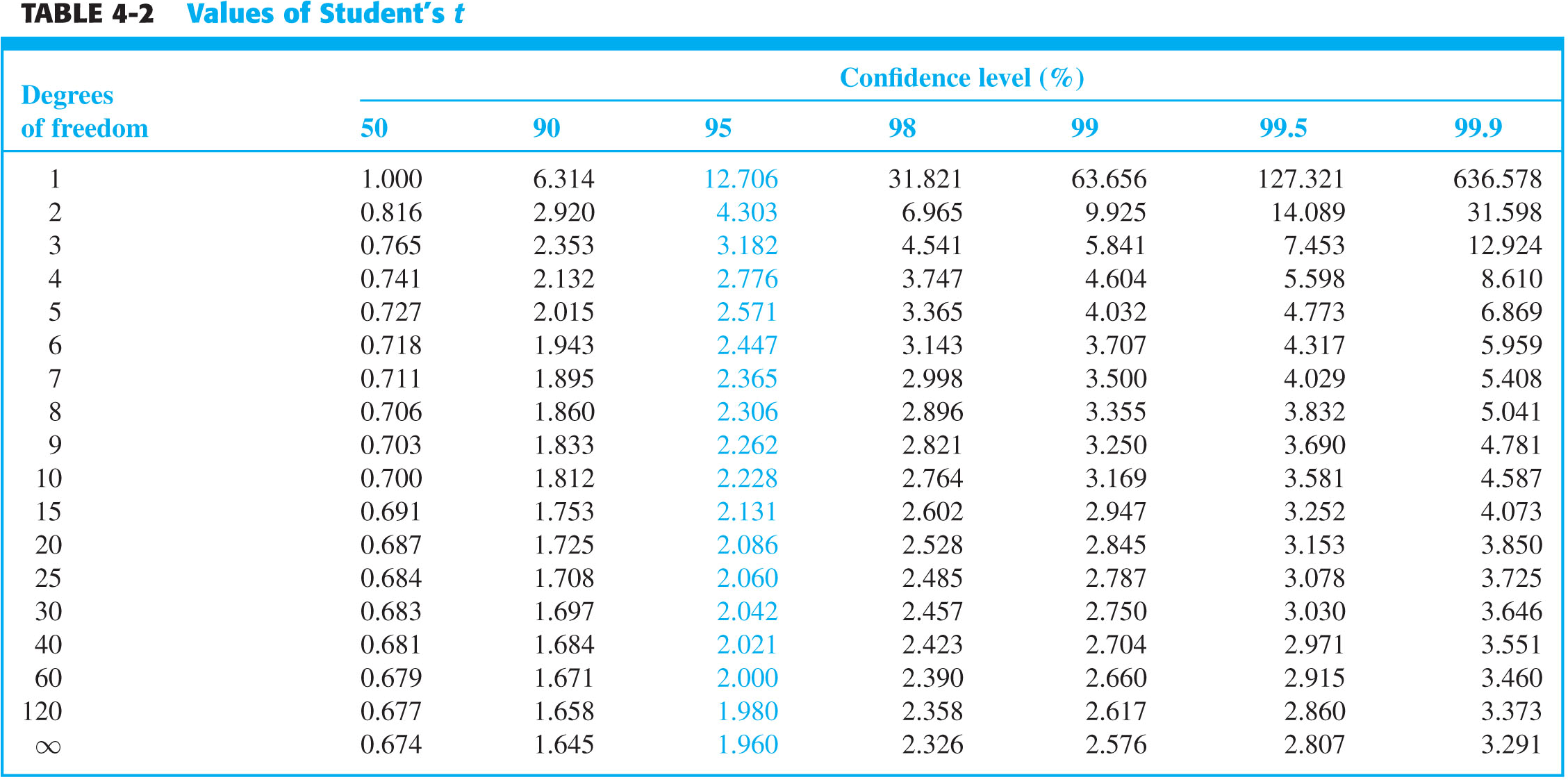
The following concentrations of titanium were detected in a sample of seawater. Find the 50% and 95% confidence intervals for the Ti content in seawater.

[Ti^4+] / nM
1.34
1.15
1.28
1.18
1.33
1.65
1.48

 

 

Discuss with your group the magnitude of the confidence intervals at each confidence level. Why would the confidence interval be smaller for a lower confidence level?

 

Example 4: T-test for comparing experimental data to a “known” value (“Case 1”)

Olympic athletes cannot have caffeine levels in their urine above concentrations of 12.00 μg/mL. Five measurements of a sample from one athlete gave a mean concentration of 12.12 μg/mL with a standard deviation of 0.09 μg/mL. At the 95% confidence level, does the athlete’s caffeine level exceed the acceptable level? (Another way of asking this is, “Does the maximum acceptable value of 12.00 μg/mL fall within the 95% confidence interval?”)

 

 

Example 5: Comparing two means of separate datasets (“Case 2”)

Return to the data in the table for Example 2. Based on the results of the F-test, use the appropriate form of the t-test to determine if the child’s BLL is decreasing significantly. Is the treatment working?

 

Assume for a moment that you obtained the opposite result for the F-test in Example 2. Discuss with your group how you would perform a t-test differently.

 

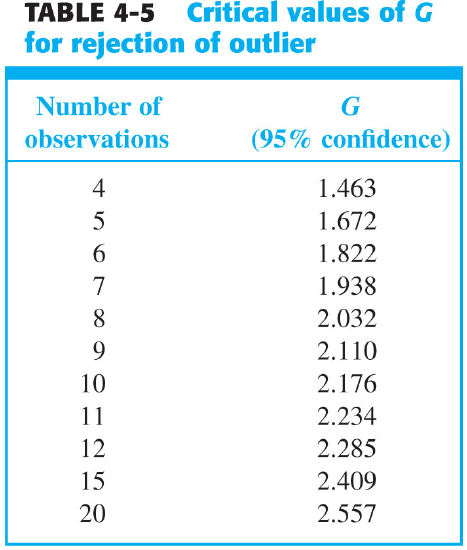
Example 6: Grubb’s test for an Outlier

A urine sample was tested five times for a metabolite of marijuana. Should any of the measurements be discarded?

Trial	Concentration (μg/L)
1	55.3
2	57.8
3	54.0
4	68.1
5	58.7

 

 

The following tables are from the Harris textbook.

\[\bar{x}=\dfrac{\sum_{i}x_i}{n} \nonumber\]

\[s = \sqrt{\dfrac{\sum_{i}(x_i-\bar{x})^2}{n-1}} \nonumber\]

\[\mu=\bar{x}\pm \dfrac{ts}{\sqrt{n}} \nonumber\]

\[G_{calc} = \dfrac{|questionable\: value - \bar{x}|}{s} \nonumber\]

\[t_{calc}=\dfrac{|\bar{x}-known\: value|}{s}\sqrt{n} \nonumber\]

\[t_{calc}=\dfrac{|\bar{x}_1-\bar{x}_2|}{\sqrt{s_1^2/n_1 + s_2^2/n_2}} \nonumber\]

\[t_{calc}=\dfrac{|\bar{x}_1-\bar{x}_2|}{s_{pooled}}\sqrt{\dfrac{n_1n_2}{n_1+n_2}} \nonumber\]

\[s_{pooled}=\sqrt{\dfrac{s_1^2(n_1-1)+s_2^2(n_2-1)}{n_1+n_2-2}} \nonumber\]

Contributors and Attributions

• Dr. Kate Mullaugh, College of Charleston ([e-mail])
• Sourced from the Analytical Sciences Digital Library